


 English (pdf)
 Article in xml format
 Article references
 Send this article by e-mail
 Cited by SciELO
  Cited by Google
  Similars in
SciELO
Similars in
SciELO  Similars in Google
 Permalink
INTRODUCTION
BPL Technology uses the electrical network as the physical means of transmission, and as the transmission standard IEEE 1901 (Home Plug AV) [1]. It also uses OFDM as a multiplexing technique and a hybrid medium access mechanism supported on CSMA/ CA and TDMA where CSMA/CA is intended for the transmission of data packets, while TDMA is used for the transmission of voice and video packets, in order to offer optimal levels of QoS [2]. Although IEEE 1901 can achieve transmission rates close to 500 Mbps, the standard lacks policies and a suitable medium access mechanism for optimal allocation of resources in the frequency and time domain [3]. This notoriously affects the provision of services over IP and the performance of the network, as the number of users and the dynamic conditions of the channel increase [4]. Therefore, the following question arises What should be done to optimize access to a BPL channel, according to the channel conditions and the requirements established by each node, in order to offer adequate QoS levels and without affecting the performance of another service? Given what was proposed, the use of weighted voting game theory, supported by the Deegan-Packel power index, is proposed as a strategy to optimize access to the BPL channel.
A BPL LAN network is a scenario in which the nodes have permanent needs to transmit, which generates disputes to access the medium, causing situations of inequity and waste of resources [5]. However, it is possible to establish an access order to the BPL channel by using Democratic systems supported on weighted voting game theory. In addition, by considering the nodes of a network as players that can work cooperatively, the probability of making a profit increases higher than that obtained from acting individually [6].
The concept of power is a very useful criterion for decision-making in various systems, and game theory makes an in-depth study of this topic. Each player can have different levels of power over the voting process, depending on the value or number of votes associated with it. However, there is not a linear dependence with the number of votes because there is a possibility that each player generates coalitions with other players [7]. Considering the above, a methodology is proposed to esta blish a scheduler per IEEE 1901 period (33.33ms), supported in the Deegan-Packel power index, to optimize the allocation of the spectrum in each node and class of service (in the time and frequency domains) estimating the allocation of the bitrate (BW) and the requirements of QoS. In addition, the use of OFDMA is proposed (Orthogonal Frequency-Division Multiple Access) [8] instead of OFDM (Orthogonal Frequency Division Multiplexing), which allows more than one node to transmit simultaneously through the BPL channel [9, 10].
The generation of the scheduler is a process managed and socialized by the node that fulfills the function of Central Coordinator (CCo) in accordance with the provisions of the IEEE 1901 standard. The Scheduler is considered as a strategy that seeks to maximize throughput and minimize collisions that occur in a multi-user scenario under a common collision domain, such as occurs in a BPL network [11].
1. METHODOLOGY
1.1 Weighted voting games
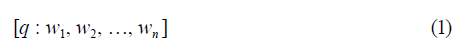
Definition: A weighted voting game is defined as a triple (N,w,q) where N={1,2,...,n} is the set of players, w = (w 1, w 2, ..., w n ) with w i > 0 for i = 1, 2, ..., n is a distribution of weights and qeR+ is the quota or majority required to win a voting process. Generally, q > ^, where T corresponds to the total sum of the weights T = w 1 + w 2 + ... + w n . A weighted voting game is represented as expressed in equation (1) [12]:
When in a voting game none of the voters has enough votes to equal the established quota, it is necessary to carry out a process of cooperation between several of them to unite their votes and establish alliances, called “coalitions”, which allow them to exceed the established quota and thereby win the voting process.
The power index is a number that is assigned to each player in order to indicate the level of power that he exercises over the game, and can be interpreted as a percentage of power for each group within the system [13]. The power indices quantify the possibilities of cooperation that each group has within the winning coalitions. The more weight, the more power. However, there are situations in which, despite the fact that the groups have different weights, they can present equal power indices [14]. In this article, the power index of Deegan-Packel will be be used as a strategy for generating a Scheduler for channel access in a BPL network.
1.2 Deegan-packel power index
The power index for a given participant in a weighted voting game is established as follows
Find the total number of minimal winning coalitions, that is, coalitions in which all participants are critical.
Find among all the g minimal coalitions, those x(P) coalitions that contain the participant P and calculate in them the inverse of the total number of voters n(x(P)) that compose it.
The index is obtained by dividing the sum of these inverses by the total number of minimal coalitions.
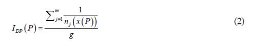
If there are g minimal coalitions and in them there are m in which the participant P appears, the power index can be calculated through the equation (2):
1.3 Algorithms for weighted voting games.
The calculation of power indices in weighted voting games is a problem that presents high levels of computational complexity when the game contains more than 20 players, due to the use of permutations within the classical algorithms [15]. Fortunately, there is a way to accomplish this process without having to inspect all possible coalitions, by using generating functions, which offer an indirect method for calculating the number of configurations of certain types. Let {a¡ } V j >0 be a sequence of real numbers, which can be represented by equation (3).
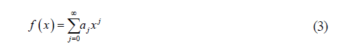
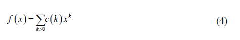
The function f(x) is called the "ordinary generating function" of the sequence {aj } V j >0. Ordinary generating functions provide a method of counting the number of elements c(k) in a finite set [16]. It is possible to represent an ordinary generating function using equation (4).
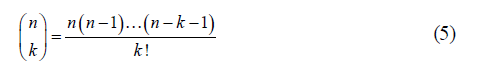
The numbThe number of subsets of k elements of N ={1,2,... n} can be determined by the equation (5) which allows to calculate the binomial coefficients.
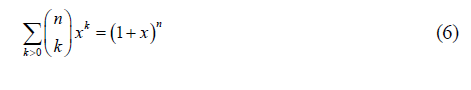
Therefore, the ordinary generating function that approximates the binomial coefficients is given by equation (6).
In Ribnikov [17] information is found that describes in greater depth the aspects related to the use and properties of the generating functions. Next, the generating functions are used as a strategy to calculate the Deegan-Packel power index in a weighted voting game (N,v), defined by v =[q; w1, w2, w„|.
1.4 Estimation of the deegan-packel power index using generating functions
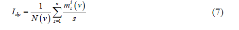
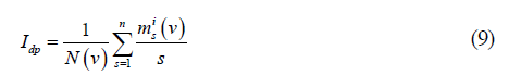
To calculate the Deegan-Packel power index in a simple game (N,v), a generating function must be used that allows calculating the cardinal of all possible coalitions, from which the winning coalitions must be chosen and finally the minimal ones (N,v) [18]. For this, it is defined msi (v) which corresponds to the number of minimal winning coalitions S to which the player belongs ieN, formed by s players. Therefore, the Deegan-Packel power index of i in a weighted voting game can be computed by equation (7).
The methodology for calculating the Deegan-Packel power index is as follows:
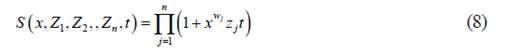
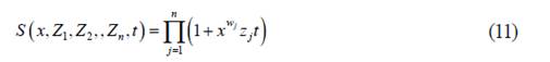
Step 1: The generating function S(x, Z1, Z2, ,Zn, t) must be calculated by equation (8).
Step 2: From the generating function, those monomials in which the power of the variable x is less than q must be eliminated, in order to determine the winning coalitions.
Step 3: Eliminate those monomials that can be divisible by some other monomial of those that are established in the group of winning coalitions. The number of mono mials of the resulting function corresponds to the number of game-winning minimal coalitions N(v).
Step 4: To obtain the Deegan-Packel value of a player i e N, simply select those terms of the resulting function in which the variable Zi appears and take the coefficient of said monomial (msi (v)). The exponent of the variable t indicates the number of players that are part of said minimal coalition (s). Taking these two elements into account, we proceed to calculate the Deegan-Packel power index for player i using equation (9).
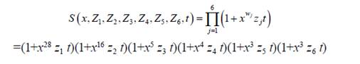
Example: Consider the weighted voting game (N, v) given from the shape which is presented in the equation (10).
Step 1: We proceed to calculate the value of q.

.Step 2: We proceed to calculate the generating function by using the equation (11).
The result is as follows:
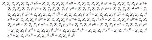
Step 3: From the generating function, those monomials in which the power of the variable x is less than q must be eliminated, in order to determine the winning coalitions. In view of the above, the resulting function is the following:
Step 4: We proceed to identify the monomials that represent the minimal coalitions. For this, those monomials that can be divisible by some other monomial of those that are established in the group of winning coalitions must be eliminated. The result of this process is the following:

The value of N(v)=6,, considering that there are 6 monomials that make up the resulting function of minimal coalitions.
Step 5: We proceed to calculate the Deegan-Packel value for each player i e N. For the case of player i = 1, the following procedure is carried out:
Those terms of the resulting function in which appears are selected.

The exponent of the variable t indicates the number of players that are part of said minimal coalition (s). Taking these two elements into account, we proceed to perform the calculation corresponding to the Deegan-Packel power index for player i=1 by using the following expression:
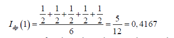
Repeating the same process for the other players, the result is as follows:
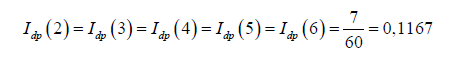
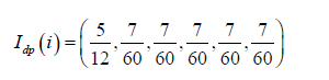
In summary, the Deegan-Packel value for the proposed game is as follows:
To facilitate future research processes related to the subject of power indices, a routine was developed in Matlab, which allows the calculation of the Deegan-Packel Power Index. The pseudocode corresponding to the routine is as follows:
\\ Routine to calculate the Deegan-Packel power index.
\\ The variables used inside the routine are:
\\ V: Vector of weights for each player
\\ q: Average value to consider the winning coalition
\\ Nj: Number of players
\\ VDeegan: Vector corresponding to the power indices for each player
Beginning
v^[28; 16; 5; 4; 3; 3];\\ The vector of weights for each player is defined Q^ceil(sum(V)/2);\\ The mean value is calculated nj^6;
\\ The Nj symbolic variables of Zj are created
Z^linspace(1 ,Nj,Nj);\\ Create a vector Z with Nj elements
Z^sym(‘Z',[N j 1]);\\ Convert vector Z to symbolic mode
PZ^ one;
For i from one until nj
PZ <- PZ*Z(i); \\ PZ corresponds to the product of the elements of Z
End_To
VDeegan^ zeros(Nj,1); \\ Initialization of the vector corresponding to the Deegan- Packel value
[or]e RandSimRepeticao(0,1E4,Nj); \\ 10000 random numbers are generated without repeating between 0 and Nj
symsx you Y
Pe zeros(Nj-1,1);
yes e y*(1+(xAV(1)*Z(1)*t*y))*(1+(xAV(2)*Z(2)*t*yA2));
PotYe 4;
For he from 3 until nj \\ Routine to establish the generating functions Bi(x) s=s*(1+(xAV(l)*Z(l)*t*yAPotY));
PotY=4Al;
End_To
s1e expand(s); \\ Perform symbolic multiplication
[cxz cy]e coeffs(s1,y); \\ Extract the coefficients of a polynomial cxz take the values of
\\ xz and c and the values of y (auxiliary variable)
c xe cxz/(PZ*tANj); \\ Extract the factor X of each monomial
[num, den]e numden(cx);
c xe num;
PotXe subs(log10(cx),x,10); \\ Evaluate the polynomial and the value of x=10 and record the total weight of each coalition
PotXe simplify(PotX); \\ Simplify values by extracting the exponents of x
TO e x.APotX;
CTe cxz./(PZ*a) ; \\ Extract the factor t from each monomial
[num, den]e numden(ct);
CTe num;
PotTe subs(log10(ct),t,10); \\ Evaluate the polynomial and the value of t=10 and record the total weight of each coalition
PotTe simplify(PotT); \\ Simplify values by extracting the exponents of t
M e find(PotX>=q); \\ The monomials that meet the condition that the power of X is >=q are selected.
PotXWine PotX(m); \\ Winning powers of X
PotTWine PotT(m); \\ Winning powers of T
Winnerse cxz(m);
nWine length(PotTWin);
For ifrom one until (nWin-1) \\ Routine to sort the PotWin vector ascending
For jfrom (i+1) until (nWin) \\ and the array of winners
Yes PotTWin(j)>PotTWin(i)
auxiliary e PotTWin(j);
PotTWin(j) e PotTWin(i);
PotTWin(i) e aux;
Aux1 e MWinners(j);
MWinners(j) e MWinners(i);
MWinners(i) e auxl;
End yes
End_To
End_To
\\ Routine to extract monomials that cannot be divided by other terms
Rie MGwinners; \\ A copy of the winning monomials is extracted
tie PotTWin;
nie length(R1); \\ The number of winning coalitions is identified
Nminimalseone;
While (n1>1)
CMinimals(Nminimals) e R1(n1); \\ Record the first minimal monomial PTMinimals(Nminimals) e t1(n1); \\ Record the power of t of the minimal monomial R e R1/R1(n1) \\ The vector R1 is divided over the last monomial in order to identify which are not divisible
[num, den] e numden(R); \\ The numerator and denominator of the previous process are extracted in each monomial
M e find(den / one); \\Those in which the denominator is different from 1 are identified R1e R1(m); \\ Those monomials that were not divisible during the process are generated.
t1et1(m);
n1elength(R1);
NminimalseNminimals+1;\\ Increase the number of minimal coalitions
End_While
n1elength(R1);
Yesn1>0
CMinimals(Nminimals) eR1(1);
PTMinimals(Nminimals) et1(n1);
End yes
\\ Calculation of the Deegan-Packel Power Index mwelength(CMinimals);\\ Mv corresponds to the total of minimal monomials For i from one until nj
R eCMinimals/Z(i);\\ Divide the vector R1 over the last monomial in order to
\\ identify which are not divisible
[num, den] e numden(R); \\ The numerator and denominator of the previous process are extracted in each monomial
M <- find(den £one); \\ Those whose denominator is different from 1 are identified R1 ^CMinimals(m);\\ Extract those monomials that were not divisible during the process. t1 ^PTMinimals(m);
n1^length(R1);
sum^0;
For j from oneuntiln1\\ Procedure that calculates the Deegan power indices Sum^sum+(1/t1(j));
End_To
VDeegan(i)=sum/Mv;
End_To
PrintVDeegan\\ Prints the vector corresponding to the power indices for each player
2. RESULTS
2.1 Proposed scenario
As a practical scenario, a LAN network made up of ten (10) BPL nodes is proposed. Each node has a BPL adapter and a traffic source. Each traffic source can generate more than one traffic class r simultaneously. For this particular case, only Data and Video traffic were considered. The 10th node will be considered as the main node or Coordinator (CCo). To estimate the channel conditions, the tool called “PLC Channel Generator (GC_PLC)” was used, written in MATLAB and developed by the PLC Group of the University of Malaga. In [19] information on the use of the GC_PLC tool is presented.
For the proposed scenario, the GC_PLC tool generated the values of 110.2 Mbps, considering typical conditions of a BPL channel. Table 1 displays that the total BW required by the nodes is 175.36 Mbps, which is higher than the total BW available in the BPL channel, thereby establishing a network insaturation state. Further, the values corresponding to the BW assigned for each node and class of traffic are presented using Nucleoulus as a strategy for the optimization of resources in the BPL network. In [20] The methodology used to estimate the assigned BW for each player is found.
Table 1 BW requested and assigned for each node of the proposed scenario
| Player or Node i | [183]Class of Service | [184]Priority Factor | [185]BW Requested | [186]Assigned BW (Nucleolus) |
|---|---|---|---|---|
| 1 | [189]Data | [190]1 | [191]11.69 | [192]7.19 |
| [195] | Video | [196]3 | [197]9.28 | [198]5.10 |
| 2 | [201]Data | [202]1 | [203]5.44 | [204]2.15 |
| [207] | Video | [208]3 | [209]13.36 | [210]8.58 |
| 3 | [213]Data | [214]1 | [215]5.22 | [216]3.37 |
| [219] | Data | [220]1 | [221]13.93 | [222]9.06 |
| 4 | [225][226] | [227] | [228] | |
| [231] | Video | [232]3 | [233]18.57 | [234]13.09 |
| 5 | [237]Data | [238]1 | [239]11.79 | [240]7.24 |
| 6 | [243]Data | [244]1 | [245]14 | [246]9.12 |
| 7 | [249]Data | [250]1 | [251]16.5 | [252]11.28 |
| [255] | Video | [256]3 | [257]16.21 | [258]11.03 |
| 8 | [261][262] | [263] | [264] | |
| [267] | Data | [268]1 | [269]11.88 | [270]7.32 |
| 9 | [273]Video | [274]3 | [275]13.45 | [276]8.65 |
| [279] | Video | [280]3 | [281]8.66 | [282]4.56 |
| 10 | [285][286] | [287] | [288] | |
| [291] | Data | [292]1 | [293]5.38 | [294]2.48 |
| [297] | [298] | Total BW | [299]175.36 | [300]110.20 |
Source: own elaboration.
2.2 Estimation of weights for each node
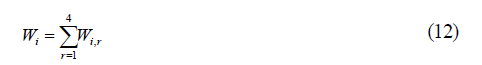
Considering that there is no evidence of a mechanism to calculate the weight of a player, in a simple weighted voting game, the following criteria were adopted to establish each of the required weights. Since each player can present more than one class of service, it is necessary to calculate a weight for each class r and player i. The value of r will be considered as the priority factor of the class of service to establish QoS mechanisms within the network. The total weight for player i can be calculated by using the equation (12) [14].
On the other hand, the weight for each class r can be calculated by using the equation (13).
Where
 corresponds to the minimum value of BW assigned among all the players whose class of service is k = r, FP
i,r
is the priority factor of the class r player i and [*] represents the operator that returns the closest largest integer of the recorded operation. Subsequently. we proceed to calculate the weights for each node according to the proposed criteria. The result of this process is recorded in Table 2.
corresponds to the minimum value of BW assigned among all the players whose class of service is k = r, FP
i,r
is the priority factor of the class r player i and [*] represents the operator that returns the closest largest integer of the recorded operation. Subsequently. we proceed to calculate the weights for each node according to the proposed criteria. The result of this process is recorded in Table 2.
Table 2 Estimated weights for each node and class of service
| Player or Node i | [313]Class of Service | [314]Priority Factor | [315]Assigned BW (Nucleolus) | [316]Total BW for Node Weight [317] [318] | [319]Overall Weight | [320] [321]||
|---|---|---|---|---|---|---|---|
| 1 | [322]Data | [323]1 | [324]7.19 | [325]12.29 | [326]4 | [327]10 | [328] [329]|
| [330] | Video | [331]3 | [332]5.10 | [333][334] | 6 | [335][336] [337] | |
| [338] | Data | [339]1 | [340]2.15 | [341][342] | 1 | [343][344] [345] | |
| 2 | [346]Video | [347]3 | [348]8.58 | [349]10.72 | [350]6 | [351]7 | [352] [353]|
| 3 | [354]Data | [355]1 | [356]3.37 | [357]3.37 | [358]2 | [359]2 | [360] [361]|
| [362] | Data | [363]1 | [364]9.06 | [365][366] | 5 | [367][368] [369] | |
| 4 | [370]Video | [371]3 | [372]13.09 | [373]22.16 | [374]9 | [375]14 | [376] [377]|
| 5 | [378]Data | [379]1 | [380]7.24 | [381]7.24 | [382]4 | [383]4 | [384] [385]|
| 6 | [386]Data | [387]1 | [388]9.12 | [389]9.12 | [390]5 | [391]5 | [392] [393]|
| 7 | [394]Data | [395]1 | [396]11.28 | [397]11.28 | [398]6 | [399]6 | [400] [401]|
| [402] | Video | [403]3 | [404]11.03 | [405][406] | 9 | [407][408] [409] | |
| 8 | [410]Data | [411]1 | [412]7.32 | [413]18.34 | [414]4 | [415]13 | [416] [417]|
| 9 | [418]Video | [419]3 | [420]8.65 | [421]8.65 | [422]6 | [423]6 | [424] [425]|
| [426] | Video | [427]3 | [428]4.56 | [429][430] | 3 | [431][432] [433] | |
| 10 | [434]Data | [435]1 | [436]2.48 | [437]7.04 | [438]2 | [439]5 | [440] [441]|
| [442] | [443] | Total BW | [444]110.20 | [445]110.2 | [446][447] | ||
Source: own elaboration.
2.3 Scheduler generation
The last objective of this article is to establish the access schedule to the medium (scheduler), by assigning the domain of time and frequency to each node i based on the power index of Deegan-Packel. This process is managed by the CCo and broadcast to each of the nodes, reducing the probability of collision and optimizing the use of the resource.
Source: own elaboration.
Figure 1 Proposed map for time and frequency distribution of a BPL channel.
Figure 1 shows the proposed map corresponding to the time and frequency dis tribution of a BPL channel, supported in OFDMA. The frequency domain is made up of the 917 subcarriers, and the time domain by 813 time slots. On this frequency-time map, the allocation of resources will be made for each node, according to the assigned BW and power index.
The proposed methodology for generating the scheduler is as follows:
Step 1: Establish the BW value assigned to each node that is part of the network, through the Nucleolus as a strategy for bandwidth optimization [21].
Step 2: Determine the total weight for each node and based on this information proceed to calculate the Deegan-Packel power index.
Table 3 Consolidated information for generating the Scheduler
| Node i | [464]Class of Serv. | [465]Priority [466] Factor | [467]BW Requested [Mbps] | [468]Assigned BW (Nucleolus) [Mbps] | [469]BW i [470] [Mbps] | [471]Weight [472] (Wi,r) | [473]Overall [474] Weight | [475]Deegan-Packel [476] Power Indices | [477]Media Access [478] Shift |
|---|---|---|---|---|---|---|---|---|---|
| 1 | [481]Data | [482]1 | [483]11.69 | [484]7.19 | [485]12.29 | [486]4 | [487]10 | [488]0.1095 | [489]3 |
| [492] | Video | [493]3 | [494]9.28 | [495]5.10 | [496][497] | 6 | [498][499] | [500] | |
| [503] | Data | [504]1 | [505]5.44 | [506]2.15 | [507][508] | 1 | [509][510] | [511] | |
| 2 | [514]Video | [515]3 | [516]13.36 | [517]8.58 | [518]10.72 | [519]6 | [520]7 | [521]0.0966 | [522]8 |
| 3 | [525]Data | [526]1 | [527]5.22 | [528]3.37 | [529]3.37 | [530]2 | [531]2 | [532]0.0613 | [533]10 |
| [536] | Data | [537]1 | [538]13.93 | [539]9.06 | [540][541] | 5 | [542][543] | [544] | |
| 4 | [547]Video | [548]3 | [549]18.57 | [550]13.09 | [551]22.16 | [552]9 | [553]14 | [554]0.1177 | [555]2 |
| 5 | [558]Data | [559]1 | [560]11.79 | [561]7.24 | [562]7.24 | [563]4 | [564]4 | [565]0.0912 | [566]9 |
| 6 | [569]Data | [570]1 | [571]14 | [572]9.12 | [573]9.12 | [574]5 | [575]5 | [576]0.1007 | [577]6 |
| 7 | [580]Data | [581]1 | [582]16.5 | [583]11.28 | [584]11.28 | [585]6 | [586]6 | [587]0.1017 | [588]4 |
| [591] | Video | [592]3 | [593]16.21 | [594]11.03 | [595][596] | 9 | [597][598] | [599] | |
| 8 | [602]Data | [603]1 | [604]11.88 | [605]7.32 | [606]18.34 | [607]4 | [608]13 | [609]0.1189 | [610]1 |
| 9 | [613]Video | [614]3 | [615]13.45 | [616]8.65 | [617]8.65 | [618]6 | [619]6 | [620]0.1017 | [621]5 |
| [624] | Video | [625]3 | [626]8.66 | [627]4.56 | [628][629] | 3 | [630][631] | [632] | |
| 10 | [635]Data | [636]1 | [637]5.38 | [638]2.48 | [639]7.04 | [640]2 | [641]5 | [642]0.1007 | [643]7 |
| [646] | [647] | Total [648] BW | [649]175.36 | [650]110.20 | [651]110.20 | [652][653] | [654] | [655] |
Source: own elaboration.
In Table 3, Steps 1 and 2 of the proposed methodology are consolidated, establishing the BW, the power index for each node, by using the Nucleolus and the Deegan-Packel Power Index, respectively.
Step 3: Using Engset's formula, estimate the recommended number of channels on which the entire BPL channel will be divided. Engset's formula is given by equation (14).
where,
P bl : Block Chance
p: ITraffic intensity generated by each node
m: Estimated number of channels
N: Number of nodes that make up the BPL network
For the proposed scenario the input parameters are:
NNodes=10;
Pl=0.01;
Ro =1.59 (BW_Requested/BW_Assigned =175.36Mbps/110.2Mbps)
[server, realPl, realPb]=find_server(NNodes, Ro, Pl)
The use of the function corresponding to the Engset formula gave a result of 10 servers, which is equivalent to the suggestion to divide the BPL channel into 10 channels with an estimated blocking probability (realPb) of 0.0208.
Step 4: Estimate the priority level of access to each of the m channels in each node, ordered from highest to lowest priority, considering the conditions of the BPL channel and the tone map present in each node. The result of this process is a matrix where the channels with the greatest intention of use by each node when requesting access to the medium are recorded. For practical purposes, numbers from 1 to 10 were randomly generated, which represent the priority order of each node to access the channel according to the possible response of the channel and the tone map generated. The result of this process is found in Table 4, which follows a matrix where the channels with the greatest intention of use by each node when requesting access to the medium are recorded.
Table 4 Channel priority per node for the proposed scenario
| Node | [678]Option 1 | [679]Option 2 | [680]Option 3 | [681]Option 4 | [682]Option 5 | [683]Option 6 | [684]Option 7 | [685]Option 8 | [686]Option 9 | [687]Option 10 |
|---|---|---|---|---|---|---|---|---|---|---|
| 1 | [690]10 | [691]2 | [692]8 | [693]3 | [694]7 | [695]6 | [696]1 | [697]9 | [698]3 | [699]7 |
| 2 | [702]6 | [703]7 | [704]5 | [705]10 | [706]7 | [707]3 | [708]9 | [709]1 | [710]2 | [711]4 |
| 3 | [714]8 | [715]4 | [716]8 | [717]10 | [718]2 | [719]5 | [720]3 | [721]7 | [722]5 | [723]1 |
| 4 | [726]3 | [727]7 | [728]6 | [729]5 | [730]2 | [731]1 | [732]4 | [733]10 | [734]8 | [735]9 |
| 5 | [738]9 | [739]4 | [740]3 | [741]8 | [742]7 | [743]1 | [744]5 | [745]2 | [746]10 | [747]6 |
| 6 | [750]5 | [751]1 | [752]9 | [753]3 | [754]6 | [755]8 | [756]9 | [757]10 | [758]2 | [759]4 |
| 7 | [762]4 | [763]5 | [764]6 | [765]9 | [766]10 | [767]1 | [768]8 | [769]3 | [770]2 | [771]7 |
| 8 | [774]1 | [775]8 | [776]4 | [777]9 | [778]2 | [779]5 | [780]6 | [781]7 | [782]3 | [783]10 |
| 9 | [786]1 | [787]3 | [788]2 | [789]4 | [790]5 | [791]7 | [792]6 | [793]8 | [794]9 | [795]10 |
| 10 | [798]8 | [799]9 | [800]6 | [801]2 | [802]1 | [803]4 | [804]5 | [805]7 | [806]10 | [807]3 |
Source: own elaboration.
Step 5: Form a Resulting Matrix (MR) in which all the parameters mentioned above are consolidated by node, and which must be ordered in descending order based on the shift assigned to access the medium. From this resulting matrix, the number of time slots equivalent to the assigned BW and the channel or channels suggested by the node are established, in an orderly manner and in accordance with the number of slots available per channel. It is important to keep in mind that the maximum number of time slots per channel is 813 and that the resource allocation can be distributed over more than one channel. The process is repeated until all nodes are assigned. Table 5 presents the resulting matrix MR, which consolidates all the information required for the construction of the scheduler.
Table 5 Resulting matrix for the proposed scenario
| Node | [814]BW [Mbps] | [815]Turn | [816]Op.1 | [817]Op.2 | [818]Op.3 | [819]Op.4 | [820]Op.5 | [821]Op.6 | [822]Op.7 | [823]Op.8 | [824]Op.9 | [825]Op.10 |
|---|---|---|---|---|---|---|---|---|---|---|---|---|
| 1 | [828]12.29 | [829]3 | [830]10 | [831]2 | [832]8 | [833]3 | [834]7 | [835]6 | [836]1 | [837]9 | [838]3 | [839]7 |
| 2 | [842]10.72 | [843]8 | [844]6 | [845]7 | [846]5 | [847]10 | [848]7 | [849]3 | [850]9 | [851]1 | [852]2 | [853]4 |
| 3 | [856]3.37 | [857]10 | [858]8 | [859]4 | [860]8 | [861]10 | [862]2 | [863]5 | [864]3 | [865]7 | [866]5 | [867]1 |
| 4 | [870]22.16 | [871]2 | [872]3 | [873]7 | [874]6 | [875]5 | [876]2 | [877]1 | [878]4 | [879]10 | [880]8 | [881]9 |
| 5 | [884]7.24 | [885]9 | [886]9 | [887]4 | [888]3 | [889]8 | [890]7 | [891]1 | [892]5 | [893]2 | [894]10 | [895]6 |
| 6 | [898]9.12 | [899]6 | [900]5 | [901]1 | [902]9 | [903]3 | [904]6 | [905]8 | [906]9 | [907]10 | [908]2 | [909]4 |
| 7 | [912]11.28 | [913]4 | [914]4 | [915]5 | [916]6 | [917]9 | [918]10 | [919]1 | [920]8 | [921]3 | [922]2 | [923]7 |
| 8 | [926]18.34 | [927]1 | [928]1 | [929]8 | [930]4 | [931]9 | [932]2 | [933]5 | [934]6 | [935]7 | [936]3 | [937]10 |
| 9 | [940]8.65 | [941]5 | [942]1 | [943]3 | [944]2 | [945]4 | [946]5 | [947]7 | [948]6 | [949]8 | [950]9 | [951]10 |
| 10 | [954]7.04 | [955]7 | [956]8 | [957]9 | [958]6 | [959]2 | [960]1 | [961]4 | [962]5 | [963]7 | [964]10 | [965]3 |
Source: own elaboration.
Next, the pseudocode of the routine that was elaborated in Matlab to carry out the generation of the scheduler based on the guidelines established in the MR matrix is presented.
\\ Routine to establish the Scheduler of a BPL network
\\ The MR Matrix is ordered in ascending order according to the turn of access to the medium.
Kmax^ NChannels+3;
For i from one until (Nj-1) For j from (i+1) until nj Yes MR(j,3) < MR(i,3) For k from one until Kmax auxiliary MR(i,k);
MR(i,k) MR(j,k);
MR(j,k) <- aux; End_To
End yes
End_To End_To
Total_Slots^ NSymbols*NChannels;
For i from one until nj \\ A Channel is the Matrix that manages channel availability AChannel(i,1) <- i; \\ A Channel(i,1) --> Node
AChannel(i,2) <- 0; \\ A Channel(i,2) --> Initial Slot End_To
K <- 0; \\ Schedule Record 1
For Ifrom one until nj
K^k+1;
\\ Estimation of the number of slots required proportional to the assigned BW. Num_Slots^ceil(Total_Slots*MR(i,2)/sum(MR(:,2)));
NPri^ 4; \\ Priority channel position
CPri^MR(i,NPri);\\ Channel Priority Okay^0;
While(ok = 0)
Schedule(k,1)^MR(i,1);\\ Node Number Schedule(k,2)^MR(i,2);\\ Assigned Bandwidth Schedule(k,3)^MR(i,3);\\ Media access shift
Yes(NSymbols >= (ACanal(CPri,2)+Num_Slots))\\ Si Slots required < slots available in the CPri channel
Schedule(k,4)^CPri;\\ Assigned Channel
Schedule(k,5)^AChannel(CPri,2)+1 ;\\ Start Slot
Schedule(k,6)^AChannel(CPri,2)+Num_Slots; \\ Final Slot
AChannel(CPri,2)^AChannel(CPri,2)+Num_Slots;\\ New Initial Slot value
Okay^ one;
Otherwise\\ On the contrary
Schedule(k,4)^CPri;\\ Assigned Channel
auxiliary <-NSymbols-AChannel(CPri,2);
Schedule(k,5)^AChannel(CPri,2)+1 ;\\ Initial Slot Part 1
Schedule(k,6)^AChannel(CPri,2)+Aux;\\ Final Slot Part 1
AChannel(CPri,2)^AChannel(CPri,2)+Aux; \\ New Initial Slot value
K^k+1;\\ New Schedule record
NPri^NPri+1;\\ Next Priority channel position
YesNPri<(NChannels+4)
CPri^MR(i,NPri);\\ New Channel Priority
Num_Slots Num_Slots-Aux;
Otherwise
ok=1;
End yes
End yes
End_While
End_To
PrintSchedule \\ Print the generated Scheduler
NNodes^10;\\ Number of nodes that are part of the LAN network
nj^NNodes; \\ Number of players = Number of nodes
\\ Estimation of HPAV eigenparameters for 60Hz
three^1/60;\\ Period of an electrical network signal at 60Hz
Tsymbol^40.96e-6;\\ Time of an OFDM symbol for HPAV
NSymbolsOloor(2*Tred/Tsymbol);\\ Number of symbols per Beacon duration
\\ HPAV (2 network cycles)^813 symbols
\\ Using the Engset formula to Calculate the number of Channels according to the Traffic Intensity
\\ and the available bandwidth.
pl^ 0.01; \\ Block chance 1% suggested.
Load_Erlangs^ 1.59; \\ Load.
server, realPl, realPb] <- find_server(NNodes, Load_Erlangs, Pl);
NChannels^ server; \\ Estimated number of channels
The result of the process corresponding to the scheduler generated for the proposed scenario is as follows:
Table 6 Scheduler of the proposed scenario
| Node | [1028]BW [Mbps] | [1029]Turn of access to the medium | [1030]Channel | [1031]Initial Slot | [1032]end slot |
|---|---|---|---|---|---|
| 8 | [1035]18.34 | [1036]1 | [1037]1 | [1038]1 | [1039]813 |
| 8 | [1042]18.34 | [1043]1 | [1044]8 | [1045]1 | [1046]541 |
| 4 | [1049]22.16 | [1050]2 | [1051]3 | [1052]1 | [1053]813 |
| 4 | [1056]22.16 | [1057]2 | [1058]6 | [1059]1 | [1060]9 |
| 4 | [1063]22.16 | [1064]2 | [1065]7 | [1066]1 | [1067]813 |
| 1 | [1070]12.29 | [1071]3 | [1072]2 | [1073]1 | [1074]94 |
| 1 | [1077]12.29 | [1078]3 | [1079]10 | [1080]1 | [1081]813 |
| 7 | [1084]11.28 | [1085]4 | [1086]4 | [1087]1 | [1088]813 |
| 7 | [1091]11.28 | [1092]4 | [1093]5 | [1094]1 | [1095]20 |
| 9 | [1098]8.65 | [1099]5 | [1100]2 | [1101]95 | [1102]733 |
| 6 | [1105]9.12 | [1106]6 | [1107]5 | [1108]21 | [1109]693 |
| 10 | [1112]7.04 | [1113]7 | [1114]8 | [1115]542 | [1116]813 |
| 10 | [1119]7.04 | [1120]7 | [1121]9 | [1122]1 | [1123]248 |
| 2 | [1126]10.72 | [1127]8 | [1128]6 | [1129]10 | [1130]800 |
| 5 | [1133]7.24 | [1134]9 | [1135]9 | [1136]249 | [1137]783 |
| 3 | [1140]3.37 | [1141]10 | [1142]2 | [1143]734 | [1144]813 |
| 3 | [1147]3.37 | [1148]10 | [1149]5 | [1150]694 | [1151]813 |
Source: own elaboration.
Table 6 shows the schedule established for the proposed scenario (scheduler), where the node, the assigned BW, the access shift to the medium, the channel or channels assigned to each node to carry out the transmission process and the time of access to the medium by means of the definition of the Slots are indicated. Start and end time for each i node.
According to the results obtained, the map of Figure 2 is presented, where it is observed that node 8 was assigned entirely to channel 1 and from slot 1 to 541 in channel 8. Node 4 was assigned entirely to channels 3 and 7 and from slot 1 to 9 on channel 6. And so on, you can verify the assignment of frequency and time assigned to the remaining nodes. Additionally, it is observed that the allocation of resources was carried out properly and without wasting slots that are part of the frequency-time spectrum.
2.4 Comparative analysis between access mechanisms to the environment represented by the MS-HPAV VS. MH-HPAV models
In order to carry out a comparative analysis between technologies, the Hybrid Model (MH-HPAV) was taken as a reference, which makes use of the CSMA/CA and TDMA media access mechanisms in a hybrid way, currently used in PLC technology (Power Line Communications) under the HomePlugAV (HPAV) standard and on the other hand, the Smart Model (MS-HPAV), which proposes OFDMA as a medium access mechanism [16]which significantly affects the network performance when the number of users increases.In light of the foregoing, it is proposed the use of the Smart Model (SM and on which the use of the Deegan-Packel power index was articulated.
During the analysis process, the Throughput, Delay and Efficiency parameters were evaluated in each of the models, based on the scenario proposed in section 2.1 and the information recorded in Table 3. Tables 7, 8 and 9 show the results obtained for each of the models, in accordance with the proposed scenario. It is important to mention that within the analysis process only the CSMA/CA, TDMA and OFDMA access mechanisms were considered due to the particularity of BPL technology.
Table 7 Results of Throughput, Delay and Efficiency forMS-HPAV(proposed) vs.MH-HPAV(current)
| [1166] | Class of Serv. | [1167]BW Requested | [1168]Assigned BW [1169] (Nucleolus) | [1170]Smart HPAV model (proposed) [1171] OFDMA + Deegan Packel | [1172][1173] | [1174] | HPAV Hybrid Model (Current) [1175] CSMA/CA+TDMA | [1176][1177] | |
| [1180] | [1181] | [Mbps] | [1182][Mbps] | [1183]Smart HPAV model (proposed) [1184] OFDMA + Deegan Packel | [1185]delay [1186] [ms] | [1187]Efficiency % | [1188]Throughput [1189] [Mbps] | [1190]delay [1191] [ms] | [1192]Efficiency % |
| [1195] | Data | [1196]11.69 | [1197]7.19 | [1198]5.99 | [1199]49.17 | [1200]51.24 | [1201]3.09 | [1202]43.72 | [1203]26.45 |
| 1 | [1206]Video | [1207]9.28 | [1208]5.1 | [1209]4.25 | [1210]49.69 | [1211]45.80 | [1212]3.21 | [1213]54.04 | [1214]34.62 |
| 2 | [1217]Data | [1218]5.44 | [1219]2.15 | [1220]1.79 | [1221]50.42 | [1222]32.90 | [1223]0.92 | [1224]37.98 | [1225]16.99 |
| [1228] | Video | [1229]13.36 | [1230]8.58 | [1231]7.15 | [1232]48.82 | [1233]53.52 | [1234]5.41 | [1235]59.83 | [1236]40.46 |
| 3 | [1239]Data | [1240]5.22 | [1241]3.37 | [1242]2.81 | [1243]50.11 | [1244]53.83 | [1245]1.45 | [1246]39.37 | [1247]27.76 |
| 4 | [1250]Data | [1251]13.93 | [1252]9.06 | [1253]7.55 | [1254]48.70 | [1255]54.20 | [1256]5.71 | [1257]50.63 | [1258]40.97 |
| [1261] | Video | [1262]18.57 | [1263]13.09 | [1264]10.91 | [1265]47.71 | [1266]58.75 | [1267]5.63 | [1268]60.42 | [1269]30.31 |
| 5 | [1272]Data | [1273]11.79 | [1274]7.24 | [1275] [1276]6.03 | [1277]49.16 | [1278]51.15 | [1279]4.56 | [1280]47.60 | [1281]38.69 |
| 6 | [1284]Data | [1285]14 | [1286]9.12 | [1287]7.60 | [1288]48.69 | [1289]54.29 | [1290]3.92 | [1291]45.91 | [1292]28.01 |
| 7 | [1295]Data | [1296]16.5 | [1297]11.28 | [1298]9.40 | [1299]48.15 | [1300]56.97 | [1301]7.11 | [1302]54.33 | [1303]43.07 |
| 8 | [1306]Video | [1307]16.21 | [1308]11.03 | [1309]9.19 | [1310]48.22 | [1311]56.69 | [1312]4.74 | [1313]58.08 | [1314]29.26 |
| [1317] | Data | [1318]11.88 | [1319]7.32 | [1320]6.10 | [1321]49.14 | [1322]51.35 | [1323]4.61 | [1324]47.73 | [1325]38.82 |
| 9 | [1328]Video | [1329]13.45 | [1330]8.65 | [1331]7.21 | [1332]48.81 | [1333]53.61 | [1334]3.72 | [1335]55.38 | [1336]27.65 |
| [1339] | Video | [1340]8.66 | [1341]4.56 | [1342]3.80 | [1343]49.82 | [1344]43.88 | [1345]2.87 | [1346]53.14 | [1347]33.17 |
| 10 | [1350]Data | [1351]5.38 | [1352]2.48 | [1353]2.07 | [1354]50.33 | [1355]38.48 | [1356]1.07 | [1357]38.36 | [1358]19.82 |
| [1361] | Total BW | [1362]175.36 | [1363]110.2 | [1364][1365] | [1366] | [1367] | [1368] | [1369] |
Source: own elaboration.
In order to assess whether the Smart Model yields better results than the Hybrid Model, the following hypotheses are proposed:
Throughput Evaluation
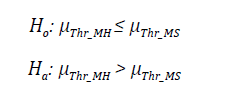
Where ¡u Thr MH and ¡u Thr MS correspond to the Throughput value obtained when using the Hybrid and Smart Models, respectively. The H o hypothesis states that the Smart Model yields better results than the Hybrid Model, as it presents an average Throughput value higher than the current method and the H a establishes the opposite condition.
Delay Evaluation
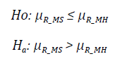
Where u R MH and u R MS correspond to the average delay obtained when using the Hybrid and Smart Models, respectively. The H o hypothesis states that the Smart Model yields better results than the Hybrid Model, as it presents a lower average delay than the current method and the H a establishes the opposite condition.
Efficiency Evaluation
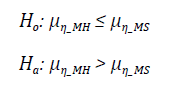
Where ¡u n MH and u n MS correspond to the average efficiency when using the Hybrid and Smart Models, respectively. The H o hypothesis states that the Smart Model yields better results than the Hybrid Model, as it presents an average efficiency higher than the current method and the H a establishes the opposite condition.
To accept or reject each of the hypotheses proposed, it is necessary to test hy potheses on the difference in means with paired sampling, using the so-called paired t-test. Making use of the miniTap statistical software, and the values recorded in Table 7; the result obtained in each of the tests is consolidated in Table 8:
Table 8 Paired t-test results for each of the established hypotheses
| Variable | [1386]Ho | [1387]Degrees of freedom | [1388]Statistical | [1389]Acceptance range [1390] ?: i < 7'( a -„.1) } | [1391]It is accepted |
|---|---|---|---|---|---|
| Throughput | [1394]p Thr_MH - p Thr_MS | [1395]14 | [1396]-6,496 | [1397](-~,1.7613) | [1398]Yes |
| Time delay | [1401]P R_MS - p R_MH | [1402]14 | [1403]-0.312 | [1404](-~,1.7613) | [1405]Yes |
| Efficiency | [1408]p n MH - p n MS | [1409]14 | [1410]-10,898 | [1411](-~,1.7613) | [1412]Yes |
Source: own elaboration.
Table 8 shows that the value of the statistic for each of the cases is within the acceptance interval, an aspect for which the H o is accepted in all three cases. In view of the above, it is concluded that with the Smart Model, which makes use of OFDMA as a mechanism to access the medium supported by the use of the Deegan-Packel power index, a better performance was obtained than the Hybrid Model (supported in CSMA/CA and TDMA), corresponding to the current state of PLC technology under the HomePlug AV standard, taking into account that for the proposed scenario, the MS-HPAV allows to achieve better levels of Throughput, delay and efficiency compared to the MH- HPAV, with 95 % confidence.
Table 9 Comparative chart MS-HPAV vs MH-HPAV.
| Variable | [1419]Model | [1420]Half % Of diference |
|---|---|---|
| [1423] | MS-HPAV | [1424]6.12 |
| Throughput | [1427][1428] | 58.3 |
| [1431] | MH-HPAV | [1432]3.87 |
| [1435] | MS-HPAV | [1436]49.13 |
| Time delay | [1439][1440] | -1.28 |
| [1443] | MH-HPAV | [1444]49.77 |
| [1447] | MS-HPAV | [1448]50.44 |
| Efficiency | [1451][1452] | 58.93 |
| [1455] | MH-HPAV | [1456]31.74 |
Source: own elaboration.
On the other hand, Table 9 presents a comparative table of the Throughput, Delay and Efficiency variables for the MS-HPAV and MH-HPAV models, based on the average value and the percentage of difference. V MS and V MH correspond to the value obtained with the Smart Model and the Hybrid Model, respectively. According to the results obtained, the following aspects can be stated:
The Throughput value achieved by MS-HPAV is 58.3 % higher than MH-HPAV, an aspect that reflects a significant improvement in the transmission processes under the proposed media access strategy.
Delay levels are reduced by 1.28 % in MS-HPAV versus MH-HPAV, which is quite favorable for transmission of services such as voice and video.
The MS-HPAV indicates an increase in system efficiency of 58.93 % compared to the current media access mechanism, optimizing resource allocation and offering adequate QoS levels to each of the nodes that are part of the network.
3. CONCLUSIONS
The use of power indices when defining the Scheduler per transmission period in a BPL network can be considered a very useful strategy. The power index represents the degree of influence that the node exerts on the network and according to the assigned value, the channel access order is established. Based on the results obtained, it was observed that the value corresponding to the power index can be estimated based on the weight reflected by the node, which depends on various factors such as: assigned BW, priority level and traffic class. At the end of the process, the CCo orders the power indices in descending order, in order to optimize the allocation of BPL channel resources, in the time and frequency domain for each node. If two nodes have equal power indices, the weight will be considered as a tiebreaker factor.
The process of calculating the power indices for each of the nodes that are part of a BPL network can be considered a problem as the number of nodes increases, because the classic algorithms make use of permutations, raising the levels of com putational complexity required. However, a routine was developed in Matlab, which allows estimating the Deegan-Packel power index through the use of generating functions, offering reduced computational and temporal complexity, to be implemented in the future in low-cost embedded systems. The development of this routine in Matlab can be considered a great contribution for future research, since it can be used in other simulation scenarios that require it.

