


 English (pdf)
 Article in xml format
 Article references
 Send this article by e-mail
 Cited by SciELO
  Cited by Google
  Similars in
SciELO
Similars in
SciELO  Similars in Google
 Permalink
Introduction
The existence of a market grants its participants -both consumers and firms- benefits known as producer and consumer surplus, which sum constitute social welfare[1]. Nevertheless, the sole existence of a market does not guarantee the maximum level of social welfare, since it may culminate in various structures, such as perfect competition, monopolistic competition, oligopoly, and monopoly.
Among all previous structures, the one that provides the maximum overall sum of benefits to society, that is the maximum social welfare, is a competitive market. Specifically, as the level of competition increases in any market the amount of production augments, the variety and quality of products or services expand, and the prices drop (Biswas & Koufopoulos, 2020; Broman & Eliasson, 2019; Nie & Yang, 2023). For example, a larger competition in the banking market promotes an increment in the quality of financial services, a reduction in their prices, a boost in the proportion of society with access to these services (Lartigue Mendoza et al., 2020), a larger rate of economic growth, and a better distribution of income (Abuselidze, 2021; Barra & Zotti, 2019; Hsieh et al., 2019).
With this in mind, the economic science has analysed the existent relationship among diverse economic variables and developed a set of mathematical instruments that permit measuring how far existing markets are from being competitive and how much market power firms have for setting prices above marginal costs in a profitable way; putting it differently, how much power firms have for choosing a price and earn more than they would do in a competitive market.
Some of these mathematical instruments have been addressed to measure the level of concentration, which refers to the number of firms and their relative participation in a given industry or market. Usually, the more concentrated a market is, the less efficiency and social welfare it achieves, punishing consumers and rewarding anti-competitive practices. In this regard, Rodríguez-Castelán et al. (2023) and Liu et al. (2022) argue that a higher concentration affects negatively firms ' productivity, given that if only a few enterprises dominate a market the competition is limited, permitting firms to operate with less pressure for improving their products, services, and processes.
On the other hand, a larger market power provokes a larger loss of consumer surplus (Adeabah & Andoh, 2019) and therefore it negatively affects social welfare (Aguilar & Portilla, 2024). For example, when commercial banks hold less market power, borrowers get better financial services, which is reflected in a larger social welfare (Wei et al., 2024).
Building on all previous arguments, it is in the best interest of market participants and governments to promote competitive markets, for all traded goods and services in their economies. Nonetheless, this path is not free of obstacles, being one of them the usual difficulty or impossibility of obtaining the value of certain variables, which are included in the formulas of these mathematical instruments, such as marginal costs and input prices.
In this line, the objective of the current paper is to help empirical economists to easily asses the competition conditions of a given market and the market power of the participant firms, by both i) explaining the integration of the main economic variables, theoretical relationships, and mathematical instruments used for this kind of assessment, and ii) exhibiting how the computation of these mathematical instruments can be simplified to require only two variables: market shares and the price elasticity of demand.
Methodologically speaking, this research makes a confrontation between economic theory and diverse technical mathematical instruments required for its application. Along the same line, it also analyzes and exposes the practical viability of the previous instruments for assessing competition conditions and market power in any market.
Thus, the questions to be answered by this research are: which theoretical relationships exist among the variables used for assessing competition conditions and market power? Given that empirically speaking the values of some variables are difficult to obtain, how can be reduced the number of variables required by the mathematical instruments used for estimating market power? Which relationships exist among the mathematical instruments used for assessing the level of concentration and the market power of a given firm or industry?
It is worth pointing out that while the discussed theoretical relationships among variables are considered neoclassical, the mathematical instruments for assessing the competitiveness of a market were developed in a parallel way during the last century. We present both the relationships between economic theory variables and mathematical instruments, as well as the existent relationships among the last ones.
On the other hand, some concentration mathematical instruments constitute special cases of the general one, such as the case of the instrument presented by Hirschman (1945) and Herfindahl (1950) some decades before the instrument introduced by Hanna & Kay (1977). Under certain assumptions, market power mathematical indicators can be derived as functions of concentration ones; these are the cases of the market power instruments introduced by Lerner (1934) and Panzar & Rosse (1977), which can be derived as functions of the concentration instrument presented by Herfindahl and Hirshman.
Analogously, the previous market power indicators -the Lerner index and the Panzar-Rosse H statistic- can be derived as a function of each other (Shaffer, 1983a). This relationship can be proved by assuming a Cournot competition with a homogeneous cost function of degree one, two inputs, a constant price elasticity of demand, and constant marginal costs (Sanchez-Cartas, 2020) or even with milder assumptions considering the previous ones but with a cost function of any degree and any amount of inputs (Domínguez & Lartigue-Mendoza, 2024).
Analogously, the previous market power indicators -the Lerner index and the Panzar-Rosse H statistic- can be derived as a function of each other (Shaffer, 1983a). This relationship can be proved by assuming a Cournot competition with a homogeneous cost function of degree one, two inputs, a constant price elasticity of demand, and constant marginal costs (Sanchez-Cartas, 2020) or even with milder assumptions considering the previous ones but with a cost function of any degree and any amount of inputs (Domínguez & Lartigue-Mendoza, 2024).
Section 2 discusses the aforementioned theoretical relationships; section 3 presents and analyses the relationships among the most recurrent mathematical instruments for assessing competition conditions and market power, as well as the techniques for estimating them; section 4 synthesizes the results; lastly, section 5 concludes.
Theoretical economic relationships
Theoretical relationships among residual demand curve, marginal revenue, and marginal cost, with competitive and non-competitive markets, national production level, and income distribution
Regardless of the market structure they belong to, firms' objective is to maximize benefits, which can be achieved through two paths. The first one is the usual maximization distance between revenues and costs, which can be achieved by taking the first derivative of the profit function -ϖ=pq-cq-2[2] with respect to the control variable (Carlton & Perloff, 2015; Motta, 2003; Tirole, 1990).
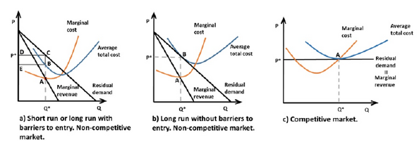
There exists a second alternative that provides the same results. This methodology is based on finding the point at which marginal revenue is identical to marginal cost -point A in Figures 2a, 2b, and 2c-; this is, the firm will increase the production till the level where one additional unit generates an additional income equal to the additional cost. Once this point is located, the firm under perfect competition will know the quantity -Q* in Figure 2c- it must offer, since the market will have already determined the price, and the firm under any other market structure -unless the firm faces a perfectly elastic demand curve-will be able to choose the price -P*- or the quantity -Q*- that correspond to this point -Figures 2a and 2b-, and the market, through the residual demand curve[3], will choose the other variable.
(1)The relationships among the curves of this Figure are discussed all along section two.
Source: Tirole (1994); Carlton & Perloff (2015).
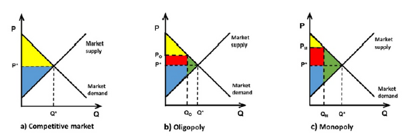
Figure 1 Consumer and producer surplus, social welfare, and social loss (1).
(1)The relationships among the curves of this Figure are discussed all along section two.
Source: Tirole (1994); Carlton & Perloff (2015).
Figure 2 Non-competitive market with and without barriers to entry and competitive market (1)
It can be seen, thus, that one of the main determinants of the level of social welfare that a market will generate is the slope of the residual demand curve a firm faces. If the residual demand curve of the good or service that a firm produces is horizontal -perfectly elastic-the price will be given, and increasing the price above market price would translate into the loss of all its customers. In this case, the price will be the lowest and the quantity the highest possible of any market structure, with these results corresponding to a perfectly competitive market structure -Figure 1a-, reaching the maximum level of social welfare that a market can breed.
On the other hand, a residual demand curve with a negative slope, which can be originated from the lack of enough competitors in the market or the existence of differentiated goods, allows the firm to set the price above the marginal cost in a profitable way; this is known as market power and can be measured by using mathematical indicators as the Lerner index -(price-marginal cost)/price-.
Given that the supply curve is nothing more than the section of the marginal cost curve that has a positive slope beginning from the average variable cost curve, setting the price above the marginal cost -before the supply curve intersects with the residual demand curve-means necessarily shrinking the supply in comparison to a perfectly competitive market -where the price will be equal to the marginal cost-.
We can then notice that a non-competitive market engenders two costs to society: a) the obtaining of a smaller production level -GDP-, generating a reduction in the level of social welfare, known as social loss -green triangles in Figures 1b and 1c-; and, b) a worsening of the income distribution, given that by placing the price above the competitive price a part of the consumer surplus is redistributed among the producers -red rectangles in Figures 1b and 1c-, who will increase their surplus -the aggregate sum of their economic rents-, thus obtaining more benefits than they would under a competitive market. In other words, a non-competitive market reallocates a fraction of the benefits belonging to milliards or millions of consumers to only a few business owners.
Relevance and relationship between barriers to entry and profitability
In general terms, provided that there are no large economies of scale, which can cause natural monopolies or oligopolies, the lack of barriers to entry -the free entry and exit of firms- will lead firms' profits to equal zero, regardless of whether the firm faces a residual demand curve with a negative slope or not.
It is worth noting that, in economic terms, a profit equal to zero means that the payment the owners of a given firm receive for the use of the production factors they provide to the firm is the market value of the same. In other words, a profit equal to zero means that total revenues are equal to total costs, and that among the latter are considered -at market value- the interest for the invested capital, the rent corresponding to any asset made available to the firm -real estate, machinery, etcetera-, and the wage of all the firm's workers, including its owners.
This way, given that through their inclusion within the costs the owners are fairly paid -at market value- for the production factors they make available to the firm, any additional profit -profit greater than zero- is known as an economic rent.
The discussion in the last three paragraphs can be observed in Figures 2a and 2b. Figure 2a may be used to illustrate both the short run of a firm in a market without barriers to entry and the long run of a firm in a market with barriers to entry. Concerning the long run, it is clear that the firm represented in Figure 2a does not belong to a competitive market, given that it faces a residual demand curve with a negative slope; has market power, since it can set the price above the marginal cost -point C is above point A-; and, captures rents, represented by the area of the rectangle with vertices on points B, C, D, and E.
With firms having free entry and exit, the existence of rents displayed in Figure 2a will appeal new firms, causing the residual demand curve, along with the corresponding marginal revenue curve, to shift to the left. This is because the more competition there is, keeping everything else constant, the less the firm will sell at any price. This can be seen in Figure 2b.
This way, even in a non-competitive market, when there exists free entry and exit of firms, two conditions are fulfilled in the long run -conditions that are fulfilled both in the long and short run in a competitive market-: a) the marginal cost is equal to -intersects- the marginal revenue -point A in Figures 2b and 2c-, and b) the average total cost curve is tangent to the residual demand curve -point B in Figure 2b and point A in Figure 2c-.
Thus, the obtaining of economic rents for a long period is a sign of the existence of barriers to entry -large economies of scale are considered natural barriers to entry-. In the following section, we present how competition conditions and market power can be easily estimated through mathematical indicators and the relationships among them.
Most recurrent mathematical instruments for assessing competition conditions and market power
The assessment of competition conditions is composed of a mixture of mathematical indicators, graphs, and intuitive discussion; all of them usually supported by the economic theory and relationships above discussed.
How profitable is a market is typically assessed through the Return to Equity -ROE- and Return to Assets -ROA- indicators. How well distributed among firms is the production and/or sales of goods or services in a given -relevant- market is assessed by concentration indicators. Lastly, how much command a firm has for setting prices above marginal costs, permitting the obtainment of economic rents, is measured by market power indicators. The last two kinds of indicators, and the relationships among them, are discussed in this section.
Concentration indicators
There exist several indexes that measure the concentration level in any given market. The most recurrent ones are the Concentration Ratio -CR-, the Hannah Kay Index, and the Herfindahl-Hirschman Index -; being the last one the standard measure in empirical research.
The Concentration Ratio
The Concentration Ratio -CR- measures the joint market share of the main firms; this way, CR3 considers the three main firms and CR4 the main four; thus, the concentration ratio for k main firms is defined as
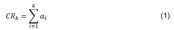
Where αj represents the market share of firm i with values between 0 and 100.
The U.S. Department of Justice and the Federal Trade Commission (2010) state market concentration can be classified according to the following ranges for CR4:
1. Perfect competition CR4 =0
2. Effective competition or monopolistic competition 0< CR4≤40.
3. Loose oligopoly or Monopolistic competition 40<CR4≤60.
4. Tight oligopoly or dominant firm with a competitive fringe CR4≤60.
One of the main criticisms to this indicator points out that it does not distinguish among the possible market share distributions of the m participant firms. For example, consider markets A and B, with the following market share distributions for the main four enterprises: market A with 40%, 20%, 10%, and 10%, and market B with 20% for each firm. In both CR4=80, although, evidently, market B is less concentrated.
The Herfindahl-Hirschman Index
The HHI formula is determined by the equation
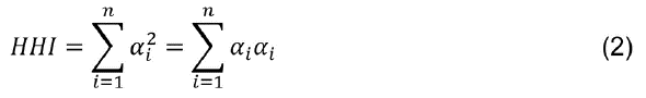
Where αi represents the market share of firm i with values between 0 and 100.
As it may be seen in the preceding formula, the HHI is the sum of the squared market share of each firm in the market under study. However, it may also be read as a weighted average of the market shares of these firms, which assigns a greater weight to larger market shares. This index may take values between 0 and 10,000, with a larger number meaning a greater market concentration.
According to the U.S. Department of Justice and the Federal Trade Commission (2010), market concentration can be determined using the following HHI ranges.
1. Deconcentrated 0 < HHI < 1500
2. Moderately concentrated 1500 ≤ HHI ≤ 2500
3. Highly concentrated 2500 < HHI
One of the main criticisms to this index is the requirement of having market share information about all participant enterprises in the analyzed market (Busu, 2020; Peleckis, 2022a, 2022b).
The Hanna Kay Index
The Hanna-Kay index is defined as
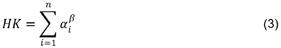
Thus, it is possible to observe that the HHI is a special case of the Hannah Kay Index when ß=2.
Market Power Indicators
Market power, understood as the ability to set the price above marginal cost in a profitable way, can be measured through the Lerner index (1934) and the Panzar-Rosse H statistic (1977), although the last one has been subject to different critiques.
The Lerner Index and its relationship with market shares and the price elasticity of demand
The Lerner index is defined as
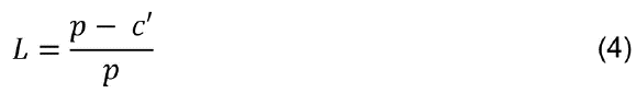
where p represents the price of a good and C’ its marginal cost. Within competitive markets price equals marginal cost -point A in Figure 2c-, therefore the Lerner index -L-total zero. The larger the market power a firm has, the greater the distance between price -point C in Figure 2a- and marginal cost -point A in Figure 2a-, with the Lerner index being closer to one.
Dickson (1979) showed, by assuming firms follow a Cournot strategic behaviour, the Lerner Index of enterprise i can be written as
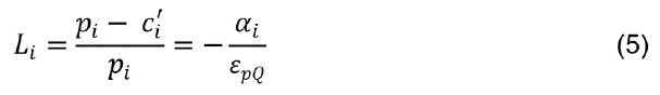
It is possible to observe on the right-hand side of equation (5) that the market power a firm possesses is an increasing function of its market share αi - and a decreasing one of the industry price elasticity of demand - ε pQ .
Multiplying both sides of equation (5) by αi and taking the sum over all firms, that is using each firm's market share as a weight for obtaining a weighted average market power, it is possible to observe that there exists a relationship between market power, the HHI, and the market price elasticity of demand Thus, the weighted average of the power to establish the price above the marginal cost -measured through the Lerner index-, observed in the totality of a market, increases with market concentration -measured with the HHI- and decreases with the market price elasticity of demand.
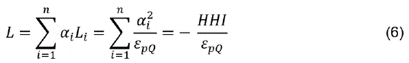
Given the constraints to obtain information on firms' marginal cost, using the right-hand side of equations (5) and (6) permits estimating the individual firms' as well as the weighted average market power observed in the whole market, respectively.
The Panzar-Rosse H statistic
Panzar and Rosse introduced a competition indicator that captures firm's revenue sensitivity to input prices. The indicator is defined as the sum of gross revenue elasticities with respect to input prices
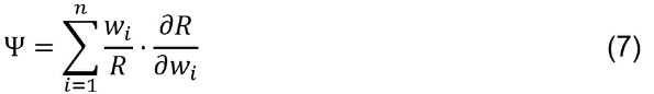
where Ψ stands for the Panzar-Rosse H statistic, Wi for input price i, and R for the revenue of the firm.
Shaffer (1983) showed that with stable residual demand curves -that is in the short run, when entry or exit of firms into the market do not occur as a response to changes in input prices-, there exists a relationship between the Lerner index of an individual firm i and its H statistics.
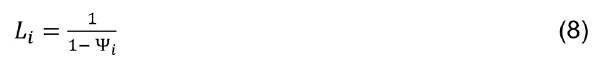
Moreover, Shaffer showed that under the Cournot assumption the industry Lerner index - L- can be estimated through
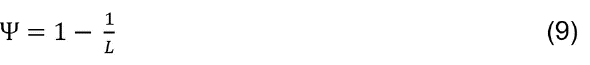
 where H is the Herfindahl-Hirschman index and the market share of firm i. Alternatively, if firms collude perfectly the relationship becomes more straightforward
 .
.
On the other hand, by assuming a Cournot competition with a homogeneous cost function of degree one, two input factors, a constant price elasticity of demand, and constant marginal costs, Sanchez-Cartas (2020) showed that the Panzar-Rosse H statistics can be easily estimated once the Lerner index is obtained.
Although the Panzar-Rosse H Statistic has been used as a market power indicator in diverse research, it has received different critiques related to the range of its possible values (Almendárez Carreón & Arteaga García, 2020; Canta et al., 2023; Cruz-García et al., 2021) and the fact that it works more like a competition indicator than a market power one (Sanchez-Cartas, 2020).
Results
Empirically speaking, the results of the current research exhibit, in section 3, how to simplify the estimation of the main mathematical indicators used for assessing the competition conditions and the market power of a given firm, industry, or market. Permitting, this way, to avoid the requirement of certain variables whose values are very difficult to obtain for empirical researchers and regulatory institutes, as marginal costs and input prices.
Specifically, we show how with only market shares it is possible to estimate concentration indicators, as the Concentration Ratio, the Herfindahl-Hirshman Index, and the Hannah-Kay Index. If the researcher gets a second variable, the price elasticity of demand, she can also estimate market power indicators, under certain assumptions, as the Lerner Index and the Panzar-Rosse H statistic.
Conclutions
This paper discusses the theoretical relationships that exist among the residual demand curve, marginal revenue, marginal cost, barriers to entry, slope of the residual demand curve, and price elasticity of demand, that determine if a market is competitive or not, and the social welfare it provides. Additionally, it integrates concentration and market power indicators into the discussed theory and resumes how they can be easily estimated.
The presented theoretical discussion concludes that if a firm holds market power, that is, the capacity to set the price above the marginal cost in a profitable manner, two conditions are fulfilled: a) it faces a residual demand curve with a negative slope; and, b) there exist barriers to entry. Thus, theoretically speaking, the attainment of economic rents for a prolonged period can be considered as an indicator of the existence of barriers to entry and market power.
While concentration indicators are functions of firms market shares, we present under which assumptions market power indicators can be simplified to functions of market shares and the industry price elasticity of demand, permitting their computation with only these two inputs.

