


 (pdf)
(pdf)


 SciELO
  Google
  SciELO
  Google
 Permalink
1. Introduction
In 2012 Arhangel’skii proposed the study in General Topology of two variants of normality; C-normality and epi-normality. Years later AlZahrani and Kalantan published a study of the behavior of these two topological properties and their relations with other normal-type properties (see [1],[6]).
At the beginning of this work we present a systematic study of the classes C-P and epi-P of topological spaces. These classes are defined in a similar way to C-normality and epi-normality, but considering an arbitrary topological property P instead of normality. We show that the classes C-P and epi-P are hereditary (additive or productive) when P is hereditary (additive or productive, respectly). Then we apply these results to study C-normal spaces; we extend the known classes of C-normal spaces by showing that they include products of locally compact spaces and locally Lindelöf spaces. We also describe some specific examples. In [6] Saeed showed the existence of a Tychonoff space which is not C-normal; we use some spaces associated with such example to prove that C-normality is not preserved under closed subspaces, unions of subspaces, continuous and closed images, and perfect preimages. This shows that the categorical behavior of C-normality is very different from normality’s categorical behavior, and answers some questions posed in [1]. We conclude the work comparing some characteristics of C-normality and epi-normality.
2. Notation
Throughout the text all spaces under consideration will be assumed to be Hausdorff. The symbol ω represents the first infinite ordinal and ω1 is the first uncountable ordinal. The continuum is denoted by c. The set of natural numbers is denoted by  and the symbol
  stands for the set of real numbers.
We say that a space X is a k-space if a set U ⊂ X is open if, an only if, U ∩ C is open in C for every compact C ⊂ X. The space X is locally Lindelöf if for each point x in X there is a neighborhood U of x which is Lindelöf. The space X is Urysohn if for each pair of different points x, y ∈ X there exist open sets U, V ⊂ X satisfying x ∈ U, y ∈ V and  ∩
∩  = ∅.
= ∅.
Given a space X, we denote as A(X) the Alexandroff duplicate X ∪ X′ of X, where X′ is a disjoint copy of X and there exist a bijective assignment x x′ from X onto X′ . Given a set U ⊂ X we choose U′ = {x′}x∈U. The topology of A(X) is defined as follows. All points of X′ are isolated and a point x ∈ X has as a basis of open neighborhoods the family of all sets of the form U ∪ U′ \ {x′}, where U is a open neighborhood of x in X.
All non stated concepts and notation can be understood as in [5].
3. The classes of epi-P and C-P spaces
The following notions describe two different ways in which we can extend the class of all topological spaces satisfying a given property.
Definition 3.1. Let P be a topological property.
A topological space X is called epi-P if there exists a bijective continuous function f: X → Y for some space Y which satisfies P.
A topological space X is C-P if there exists a bijective function f : X → Y , where Y has property P, and f ↾C: C → f(C) is a homeomorphism for each compact C ⊂ X.
Given a topological property P, since every bijective continuous function defined on a compact Hausdorff space is a homeomorphism onto its image, all epi-P spaces are C-P. The other implication is not always true, for example when P coincides with normality (see Example 6.5). The following result gives us a condition under which these two notions are equivalent; the proof follows since for a k-space X a function f : X → Y is continuous if, and only if, f ↾C is continuous for each compact C ⊂ X (see [5, Theorem 3.3.21]).
Proposition 3.2. If P is a topological property and X is a k-space, then X is C-P if, and only if, X is epi-P.
The classes C-P and epi-P can coincide, for example when a space X satisfies P if, and only if, every compact subset of X is metrizable.
If a topological property P implies another topological property Q, then all epi-P (C-P) spaces are epi-Q (C-Q). Besides, if P and Q are different properties, the class of epi-P spaces and the class of epi-Q spaces can coincide; for example, when Q is the class of epi-P spaces the class of epi-P spaces coincides with the class of epi-Q spaces. Similarly, the classes C-P and C-Q can coincide, as we will show now.
Theorem 3.3. If P is a topological property, the class of C-P spaces and the class of C-(C-P) spaces coincide.
Proof. It is sufficient to prove that every C-(C-P) space is C-P. Suppose that there exists a bijective function f : X → Y , where Y is C-P and f ↾C: C → f(C) is a homeomorphism for each compact subspace C ⊂ X; we shall prove that X is C-P. As Y is C-P, there exists a space Z with property P and a bijective function g : Y → Z such that g ↾D: D → g(D) is a homeomorphism for each compact subspace D ⊂ Y . We claim that g ◦ f witnesses that X is C-P. Indeed, let C ⊂ X compact. Since f ↾C: C → f(C) is a homeomorphism, the space D = f(C) is compact. It follows that g ↾D: D → g(D) is a homeomorphism. Thus (g ◦ f) ↾C = (g ↾D) ◦ (f ↾C) : C → g ◦ f(C) is a homeomorphism and, since Z has property P, we conclude that X is C-P.
In what follows we will analyze some properties of the classes epi-P and C-P inherited from the property P.
Theorem 3.4. If a property P is hereditary, then the classes C-P and epi-P are closed under arbitrary subspaces.
Proof. We will show the case of C-P spaces; the proof for the epi-P spaces is similar. Let A be a subset of X. As X is a C-P space, there exists a bijective function f : X → Y , where Y has property P, such that f ↾C : C → f(C) is a homeomorphism for each compact subspace C ⊂ X. Since the property P is hereditary, the space f(A) has property P. It is clear that f ↾A: A → f(A) is bijective. Since any compact subspace of A is compact in X, the restriction (f ↾A) ↾C = f ↾C is a homeomorphism for each compact subspace C ⊂ A. Thus A is C-P.
Theorem 3.5. If κ is a cardinal and P is a κ-productive property, then the classes C-P and epi-P are closed under products of κ-factors.
Proof. We will prove the result for the class C-P; the case of the class epi-P is similar. Let {Xs}s∈S be a family of C-P spaces where S has cardinality κ. For each s ∈ S let fs: Xs → Ys be a bijective function for some Ys with property P such that fs ↾Cs: Cs → fs(Cs) is a homeomorphism for each compact subspace Cs ⊂ Xs. Note that f = ∏s∈Sfs: ∏s∈S Xs → ∏ s∈SYs is bijective. Besides, as P is a κ-productive property, it follows that ∏s∈S Ys has property P. Given a compact set C ⊂ ∏s∈S Xs, notice that D = ∏s∈Sπs(C) is compact, and so the function f ↾D= ∏s∈Sfs ↾πs(C)= D → f(D) is a homeomorphism; consequently, f ↾C: C → f(C) also is a homeomorphism. Thus, the product ∏s∈SXs is C-P.
Theorem 3.6. If P is a κ-aditive property, then the classes C-P and epi-P are closed under disjoint sums of κ-factors.
Proof. We will prove the result for the class of C-P spaces, the other case is similar. Let {Xs}s∈S be a family of spaces C-P where |S| = κ. For each s ∈ S, let fs: Xs → Ys be a bijective function for some space Ys with property P such that fs ↾Cs: Cs → fs(Cs) is a homeomorphism for each compact subspace Cs ⊂ Xs. As P is a κ additive property, it follows that ⊕s∈SYs has property P. Besides, the function ⊕s∈Sfs: ⊕s∈SXs → ⊕s∈SYs is bijective. Now let C ⊂ ⊕
s∈SXs be a compact space, then the set S0 = {s ∈ S : C ∩ Xs ∅} is finite and Cs = C ∩ Xs is compact for each s ∈ S0. Then (⊕s∈Sfs) ↾C = ⊕s∈S0fs ↾Cs is a homeomorphism, because fs ↾Cs is a homeomorphism for each s ∈ S0. Thus, the disjoint sum ⊕s∈SXs is C-P.
By an argument similar to the one used in the proof of Theorem 3.5 we can prove the following result.
Proposition 3.7. Consider two properties P and Q such that X × Y has P when X has P and Y has Q. Then X × Y is C-P when X is C-P and Y is C-Q.
Theorem 3.8. Let P be a property preserved under Alexandroff duplicates; then A(X) is C-P (epi-P) whenever X is C-P (epi-P).
Proof. We will show the case of C-P spaces; the case for the epi-P spaces is similar. Let X be a C-P space; then, there exists a space Y with property P and a bijective function f : X → Y such that f ↾C: C → f(C) is a homeomorphism for each compact subspace C ⊂ X. Consider the Alexandroff duplicated A(X) and A(Y ) of X and Y , respectly. Since Y has P, the space A(Y ) also has P. Define F : A(X) → A(Y ) by F(x) = f(x) and F(x′) = f(x)′ for each x ∈ X, the natural function induced by f. Notice that F is a bijective function. Let C ⊂ A(X) be a compact subspace. We shall prove that F ↾C: C → F(C) is a homeomorphism. Let p : A(X) → X be the function given by p(x) = p(x′) = x, for each x ∈ X. Observe that p is continuous. For the compact set D = p(C) we have that g = f ↾D is bijective and continuous. It is easy to verify that the natural function G : A(D) → A(g(D)) induced by g, given by G(x) = g(x) and G(x′) = g(x)′ for each x ∈ D, also is bijective and continuous. As A(D) is compact, the function G is a homeomorphism. We know that C ⊂ A(D) ⊂ A(X), thus F ↾C = G ↾C also is a homeomorphism.
We consider now the following well known construction. Let X be an arbitrary space. Take kX = X. Define a topology on kX as follows. A set of kX is open if, and only if, its intersection with any compact subspace C of X is open in C. Then the space kX endowed with this topology is a k-space, has exactly the same compact subspaces that X, and induces the same topology that X on these compact subspaces. From these observations it is easy to conclude the following.
Proposition 3.9. Let Pbe a topological property. A space X is C-Pif, and only if, kX is C-P.
4. C-normal spaces
In this text we will be particularly interested in C-normality and some related properties. Notice that all epi-normal spaces, all C-compact spaces and all C-metrizable spaces are C-normal. We will provide another classes of spaces which are C-normal.
As is stated in Exercise 3.3.D from [5], every locally compact space is epi-compact, so we can apply Theorem 3.5 to obtain the following corollary.
Corollary 4.1. If {Xs}s∈Sis a family of locally compact spaces, then the product ∏s∈SXsis epi-compact.
Example 4.2. The space of real numbers  is locally compact, because of Corollary 4.1 the product
  is C-normal, for any set S. Moreover, if
  is the Sorgenfrey line, then
  admits a bijective continuous function onto
  , so we can apply Theorem 3.3 to see that
  is C-normal. However,
  is not normal when the set S is not countable (see [5, Exercise 2.3.E]) and
  is not normal when S has at least two elements (see [5, Example 2.3.12]).
Now we will deal with a notion more general than locally compactness, local Lindelöfness, in order to get more examples of C-normal spaces.
Theorem 4.3. If X is regular and locally Lindelöf, then X is epi-Lindelöf.
Proof. We must prove that X admits a bijective and continuous function onto a Lindelöf space. Let Y = X ∪ {y} where y X. We define a topology in Y in the following way. The topology of Y is the minimal topology on Y which satisfies the following conditions:
It contains the topology of X.
It contains each set U ⊂ Y such that y ∈ U and whose complement Y \U, is closed in X and has a neighborhood in X whose closure in X has the Lindelöf property.
As X is regular and locally Lindelöf, the space Y is T1. We will verify now that Y is regular. Given A ⊂ X, along this proof A always refers to the closure of A in X. Take a point x ∈ Y and a neighborhood U of x in Y . If x  y, since X is regular, we can suppose that U ⊂ X and
  is Lindelöf. By the regularity of X, there exists an open neighborhood V of x such that x ∈ V ⊂
  ⊂ U. Notice that
  is closed in Y . If x = y we can suppose that F = Y \ U is closed in X and has a neighborhood V in X whose closure
  in X has the Lindelöf property. As
  is normal, there exists an open set W in X such that F ⊂ W ⊂
  ⊂ V ⊂
⊂ V ⊂  . It follows that
  is closed in Y , and if O = Y \
  , then y ∈ O ⊂ {y} ∪
  ⊂ Y \ W ⊂ Y \ F = U, where {y} ∪
  is the closure of O in Y . Thus, the space Y is regular.
It is easy to verify that Y is Lindelöf. Fix x ∈ X and consider the space Z which is obtained from Y identifying the points x and y, and let q : Y → Z be the quotient function associated with this identification. As Y is normal and q only identifies a closed set, the space Z is regular. Since q is continuous, the space Z is Lindelöf. Finally, is clear that the function q ↾X: X → Z is bijective, and hence this function witnesses that X is epi-Lindelöf.
We now describe some examples of locally Lindelöf spaces, and hence C-normal spaces, which are neither locally compact nor normal.
Example 4.4. Let X be a locally compact not normal space and let Y be a Lindelöf not locally compact space. Consider the space X ×Y . Note that X ×Y is not normal, because it has a closed subspace homeomorphic to X which is not normal. Observe that X × Y is not locally compact, because it has a closed subspace homeomorphic to Y which is not locally compact. However, the product X ×Y is locally Lindelöf, because the product of a compact space and a Lindelöf space is always Lindelöf. Thus, Theorem 4.3 implies that X × Y is C-normal. As a particular case, we can take X as the deleted Tychonoff plank and Y as the Sorgenfrey line.
Example 4.5. Consider the following variant of a Ψ-space.Let A be a maximal family of uncountable subsets ofω1such thatA ∩ B is countable for eachA, B ∈ A. It is easy to deduce from the maximality of A that |A| ≥ ω2. Consider the space Ψω1 (A) = ω1 ∪ A, where each point in ω1is isolated and every A ∈ A has as a basis of open neighborhoods the family {A \ C : C ∈ [ω1]<ω1}. It follows immediately from the definition that Ψω1 (A)is locally Lindelöf and not locally compact.
We will prove that Ψω1(A) is not normal. Suppose on the contrary, that Ψω1(A) is normal. Let {Aα}α<ω1 be a partition of A in nonempty subsets and fix Aα∈ Aα for each α < ω1. Given α < ω1, because of the normality of Ψω1(A) we can choose an uncountable subset Bα of ω1 such that the subsets Aα∪ Bα and (A \ Aα) ∪ (ω1\ Bα) form a partition of Ψω1(A) in open sets. We will construct a subset {xα}α<ω1 of ω1 recursively as follows. Fix x0 ∈ A0, and if {xα}α<β is defined for some β < ω1, fix xβ ∈ Aβ\∪α<β({xα}∪ Bα). Consider the uncountable set B = {xα}α<ω1 ; then the maximality of A implies that A∩B is uncountable for some A ∈ A. We know that A ∈ Aγ for some γ < ω1. Since {A} ∪ Bγ is open, we must have that (A ∩ B) \ Bγ⊂ A \ Bγ is countable, and hence (A ∩ B) \ Bγ ⊂ {xα}α<β for some γ >< β < ω1. Since A ∩ B is uncountable, we can suppose that β is such that xβ∈ A ∩ B. However, the construction implies that xβ Bγ, which is not possible. Thus, the space Ψω1(A) is not normal.
Question 4.6. Is there a locally normal regular space X which is not C-normal?
Proposition 4.7. If any countable subspace of X is discrete, then X is C-normal.
Proof. By [1, Corollary 1.4] it is sufficient to verify that all compact subsets of X are finite; namely, under such conditions any bijection onto a discrete space witnesses the C-normality of X. Let A ⊂ X infinite. Take B ⊂ A infinite and countable. Note that B is closed in X because B ∪ {x} is discrete for each x ∈ X. As B is closed, discrete and infinite, it follows that A is not compact.
We now describe an example of a space in which all countable subsets are discrete, and hence a C-normal space, but which is not normal. This example was obtained by Shakhmatov (see [3, Example 1.2.5]).
Example 4.8. Let Ic be the Tychonoff cube of weight c. Let
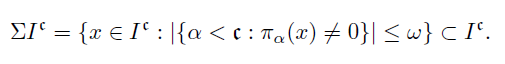
Observe that |ΣIc| =c, and take an enumeration {xα}α<c of the elements of ΣIc where each element appears c-many times. Moreover, take an enumeration {Aα}α<c of the elements from [c]≤ω where each element appears c-many times. For each α <c define a point yα Ic by:
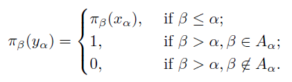
As it is proved in [3, Example 1.2.5], the space Y = {yα}α<c ⊂ Ic is dense in Ic, pseudocompact, and every countable subset of Y is discrete. As Y is pseudocompact but not countably compact, we conclude from [5, Theorem 3.10.21] that Y is not normal.
5. Operations with C-normal spaces
In [6] Saeed showed the existence of a Tychonoff space which is not C-normal. Such example is constructed as follows: Let 2ω1 be the Cantor cube of size ω1; the product of ω1-many copies of the discrete two points space. Now consider the subspace
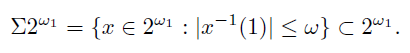
Then the product 2ω1 × Σ2ω1 is Tychonoff but not C-normal (see [6, Example 8]). This example provides us a compact space and a normal space whose product is not C-normal, so C-normality is not a productive property. However, we still do not know the answer to the following question.
Question 5.1. Is there a C-normal space X such that its square is not C-normal?
We know that normality is preserved under closed subspaces and closed continuous images. In the following examples we will show that C-normality is not necessary preserved in these cases.
Example 5.2. There exists an epi-compact space containing a closed subspace which is not C-normal.
Proof. Consider the cartesian product Y = 2ω1 × 2ω1 endowed with the product topology, and the cartesian product X = 2ω1 × 2ω1 endowed with the topology obtained from the product topology by adding 2ω1 × Σ2ω1 and its complement as open sets. Notice that X is epi-normal; indeed, the identity function id : X → Y is continuous and Y is compact. It is clear that 2ω1 ×Σ2ω1 is closed in X. Moreover, the topology on 2ω1 ×Σ2ω1 inherited from X coincides with the topology inherited from Y . Thus, 2ω1 × Σ2ω1 is a closed subspace of X which is not C-normal.
Example 5.3. There exists an epi-compact space admitting a closed continuous image which is not C-normal.
Proof. Take the spaces X and Y as in Example 5.2. Now consider the function f : X → Y given by:
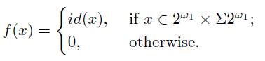
Notice that f is continuous and f(X) = 2ω1 × Σ2ω1 . Besides, if F is closed in X, then either f(F) = F ∩(2ω1 ×Σ2ω1 ) or f(F) = (F ∩(2ω1 ×Σ2ω1))∪ {0}. It follows that f is a closed function. Finally, we know that X is epi-compact and f(X) is not C-normal.
Any closed continuous function is quotient; from the previous result we conclude that C-normality is not preserved under quotient functions. It happens that C-normality is also not preserved under open perfect preimages. Indeed, take the proyection π : 2ω1×Σ2ω1 → Σ2ω1 on the second factor. As 2ω1 is compact, it follows from [5, Theorem 3.7.1.] that the function π is perfect. However, the space Σ2ω1 is C-normal while 2ω1×Σ2ω1 = π−1 (Σ2ω1) is not C-normal.
Question 5.4. Suppose X × K is C-normal for some compact K. Is it true that X is C-normal?
We will prove now that C-normality is not preserved under the union of two arbitrary subspaces; we will use an example obtained in [4].
Example 5.5. There exists a non-C-normal space which is the union of a compact sub-space and a locally compact subspace.
Proof. Consider the topological product (ω1 + 1)×[0, 1], the subspace R = {ω1} ×(0, 1), the space X = ( (ω1 + 1) × [0, 1]) \ R, and the space Y = X × (ω1 + 1). Then the space Y is not C-normal (see [4]). Now, take A = (ω1 + 1) × {0, 1} × (ω1 + 1) and B = (ω1 + 1) × (0, 1) × (ω1 + 1). Clearly A is compact, B is locally compact, and Y = A ∪ B.
Question 5.6. Is there a non-C-normal Tychonoff space X which is the union of two C-normal closed subspaces?
Now we will answer in the positive the following question which is attributed to Arhangel’skii in [7]; Is there a normal space which is not C-paracompact?
Example 5.7. There exists a normal space which is not C-paracompact.
Proof. Consider the normal space Σ2ω1 . We claim that Σ2ω1 is not C-paracompact. Suppose that the space Σ2ω1 is C-paracompact. Since 2ω1 is C-compact, we can apply Proposition 3.7 and the fact that the product of a compact space and a paracompact space is paracompact (see [5, Theorem 5.1.36]), to conclude that 2ω1 × Σ2ω1 is C-paracompact and thus C-normal; which we know is not true. Thus, the space Σ2ω1 is not C-paracompact.
Note that using the space described in examples 5.2 and 5.7 we can conclude that C-paracompactness is not inherited by closed subspaces. It is worth to mention that Example 5.7 also provides an epi-normal space which is not C-paracompact. This answers another question from [7].
6. Epi-normal spaces
It follows from Examples 5.2, 5.3 and 5.5 that epi-normality is not necessarily preserved under closed subspaces, unions, products, continuous and closed images, and inverse images of perfect functions. Now we will analyze other properties of epi-normal spaces.
Proposition 6.1.
Let X be an epi-normal space. If g : C →  is a continuous function, where C ⊂ X is compact, then there exists a continuous function
 : X →
: X →  such that
 ↾C = g.
Proof. Let f: X → Y be bijective and continuous, for some normal space Y . Notice that f ↾C: C → f(C) is a homeomorphism. As Y is normal, the function h = g ◦ (f ↾C )−1: f(C) →  admits a continuous extension
  : Y →
: Y →  . We consider the continuous function
  =
=  ◦ f : X →
  . Notice that

is the required extension of g.
Corollary 6.2. If X is epi-normal, then X is Urysohn.
Proof. Given two distinct points x, y ∈ X, by Proposition 6.1 we can take a continuous function f : X →  such that f(x) = 2 and f(y) = 5. Then the open subsets U = f−1 ((1, 3)) and V = f−1 ((4, 6)) of X have disjoint closures and contain x and y, respectively.
The following example shows that, in general, epi-normal spaces are not necessary regular.
Example 6.3. Let X =  and consider the sequence A =
  Define a topology in X as the family of all sets of the form U \ B where B ⊂ A and U is open in the usual topology of
 . Clearly X is epi-normal, because its topology is finer than the usual topology. However, the space X is not regular, because {0} and A cannot be separated by disjoint open subsets.
Example 6.4. There exists a space X which is neither C-normal nor Urysohn, but which is the union of two epi-normal closed subspaces.
Proof. Let X = ( \ {0}) ∪ {x1, x2}, where x1 and x2 do not belong to
  . Define a topology in X as follows. The space
  \ {0} endowed with its usual topology is an open subspace of X. Besides, for each i = 1, 2 the point xi has as a basis of open neighborhoods the family of all sets of the form

where n ∈  . Note that x1 and x2 cannot be separated using neighborhoods with disjoint closures, thus X is not Urysohn. As an application of Corollary 6.2 we obtain that X is not epi-normal. Observe that X is Fréchet-Urysohn, so we can apply Proposition 3.2 to conclude that X is not C-normal. Choose i ∈ {1, 2}. Let Ai = {(x, y) : (−1)iy ≥ 0}\{0}. Note that Ai ∪ {xi} admits a bijective continuous function onto the subspace Ai ∪ {0} of
  and hence is epi-normal. Therefore, the space X = (A1 ∪ {x1}) ∪ (A2 ∪ {x2}) is the union of two closed epi-normal subspaces.
It happens that C-normal spaces are not necessarily Urysohn, as the following example shows.
Example 6.5. There exists a C-normal space which is not Urysohn.
Proof. Consider the space ω1 with the discrete topology. Let L = ω1+1 endowed with the following topology. The space ω1 is open in L and ω1 has as a basis of open neighborhoods the family of all sets (α, ω1], where α < ω1. Consider the open subspace O = L × ω1 of L × L. Let {A1, A2} be a partition of ω1 into uncountable sets. Consider the space X = O ∪ {x1, x2}, where x1, x2 L×L, endowed with the following topology. The space O is open in X and, for i ∈ {1, 2} the point xi
has as a basis of open neighborhoods the family of all sets of the form (U ∩ (Ai × ω1)) ∪ {xi} where U is a neigborhood of (ω1, ω1) in L × L. Note that X is Hausdorff. Besides, the space X is not Urysohn because the points x1 and x2 cannot be separated by open sets in X with disjoint closures. However, if we take Y = O ⊕ {x1} ⊕ {x2}, then Y is normal and the restriction of the identity function from X onto Y to each compact subspace is a homeomorphism, that is, the space X is C-normal.
L×L, endowed with the following topology. The space O is open in X and, for i ∈ {1, 2} the point xi
has as a basis of open neighborhoods the family of all sets of the form (U ∩ (Ai × ω1)) ∪ {xi} where U is a neigborhood of (ω1, ω1) in L × L. Note that X is Hausdorff. Besides, the space X is not Urysohn because the points x1 and x2 cannot be separated by open sets in X with disjoint closures. However, if we take Y = O ⊕ {x1} ⊕ {x2}, then Y is normal and the restriction of the identity function from X onto Y to each compact subspace is a homeomorphism, that is, the space X is C-normal.

