1. Introduction

A thermoelastic system describes the behaviour of elastic bodies exposed to heat flow (source of dissipation). The thermoelastic system described herein considers a thermal effect and is a modified version of the Lamé system, which describes the displacement in elastic bodies.

To barely understand a thermoelastic system, one must (i) refer to the theory of elasticity and comprehend the equation of elasticity considering multiple conditions of the elastic medium and, (ii) understand the modelling in heat theory.

Elastic model. For an introduction to the theory of elasticity see [⁶], [¹⁸], [²⁰]. In Narukawa [¹³] the author includes a pleasant explanation about how an elastic model can be obtained from the first principles. Let us briefly outline the main ideas presented in [¹³] with this respect. It is known, from the theory of elasticity, that equation (1.1) describes the displacement u(x, t) = {u_i(x, t)}₁≤i≤n

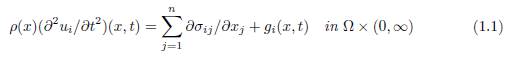
where ρ(x), σ_ij(1 ≤ i, j ≤ n) and g(x, t) = {g_i(x, t)}₁≤i≤n denote the density, the stress tensor and the external force, respectively.

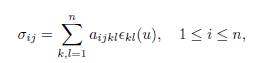
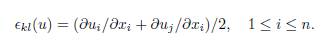
between the stress tensor σ_ij and the linearized strain tensor

The functions a_ijkl, called coefficients of elasticity, depend on t and x but are independent of the strain tensors. If the coefficients of elasticity are constant and if the medium is isotropic, that is, if its elastic properties are the same in all directions, then

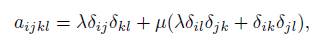
where {δ_ij} is the Kronecker tensor and λ and µ are constant Lamé coefficients. When the density is equal to a constant ρ₀, the system (1.1) can be written as

Heat conduction model. It is known that heat conservation equation is given by

where q and θ are the heat flux and temperature, respectively. Fourier’s law is the most simple empirical law widely used to explain heat conduction phenomena. It states that the heat flux vector is proportional to the negative gradient of temperature in direction of the energy flow. In isotropic materials, this law corresponds to:

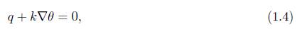
where the constant k > 0 is called thermal conductivity. However, as it is well-known, Fourier’s law entails the physical paradox of infinite velocity of heat transmission. In particular, it is important to say that Cattaneo’s Law inhibits the physical paradox of the infinite speed of propagation of signals, but that it maintains the essential of a heat conduction process which presents some drawbacks at the level of physical experiments. For instance, in dielectric crystals at low temperatures, the thermal disturbances propa-gate at a finite velocity. From these phenomena, the need to consider other theories of heat conduction emerges. A generalization of Fourier law, on which this article is based, was proposed by Cattaneo in 1948 [²]; it is described as

where τ₀ ≥ 0 is called relaxation time. Here the time derivative term forces the heat propagation to have finite velocity, whenever τ₀ > 0. This model is widely accepted as an alternative of Fourier’s law which inhibits the above mentioned physical paradox. It is clear that in the case τ₀ = 0, (1.5) coincides with Fourier’s law (1.4).

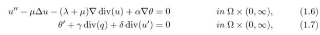
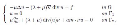
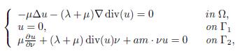
Thermoelastic model. The system we proposed to study is defined by a bounded n-dimensional domain Ω, n ≥ 2, homogeneous, isotropic and with border Γ = ∂Ω of class C², where the equations of thermoelasticity in Ω are of the form:

with u = u(x, t) ∈ ℝ ⁿ being the displacement vector, θ = θ(x, t) ∈ R the difference in temperature over time t with respect to a reference temperature measured in t = 0, q = q(x, t) the heat flow, x ∈ ℝ ⁿ and t ∈ ℝ ⁺ ∪ {0} the spatial and temporal variables, respectively. On the other hand, Δu = (Δu₁, . . . ,Δu_n), div(u) = , and ∇ represent the Laplacian operator, divergence, and gradient for spatial variables, respectively. The symbol (^′) denotes the derivative with respect to the temporal variable. The constants λ, µ > 0 are the Lamé constants, and α and δ are positive coupling parameters. The therms α∇θ and δ div(u^′) are added to equations (1.2) and (1.3), respectively, in such a way that the temperature gradient acts as a force on the elastic component, while the wave pressure acts as a heat source in the heat equation.

Results on the exponential stability of solutions for system (1.6)-(1.7) are widely known in the case of n = 1 with different boundary conditions, see for instance [⁴]. When considering n ≥ 2, one finds that depending on boundary conditions, the decay of solutions can be exponential or polynomial. In fact, the usual technique considers two behaviours at the boundary: one to define a dissipative term and another to fix the variable u, obtaining thus exponential or polynomial decays according to the type of dissipation, see for instance [⁹], [¹¹], [¹⁰]. This technique was initially applied to models that do not involve a heat flow, see for instance [⁷], [⁸], [²⁰]. It should also be noted that many of these results have occurred in the case where the law of heat flow is modeled by Fourier’s law (1.4). Some exponential stability results for the linear and non-linear thermoelastic systems with Fourier’s flow law in 1, 2 and 3 dimensions can be found in [¹⁵].

Regarding the thermoelastic systems with heat flow given by Cattaneo (1.5), also known as thermoelastic systems with second sound, several results have been published. Chan-drasekharaiah [³] presents the first references about thermoelastic systems with second sound and, Tarabek in [¹⁹] establishes the existence of solutions for small data in the case of problems defined in bounded and unbounded one-dimensional domains. It has also been established in [¹⁹] that the solutions converge to equilibrium when t → ∞, but no results are presented for the study of decay rates. Later, Racke [¹⁷] establishes uniform decay for linear and nonlinear initial value problems in dimension n = 1. In addition, the author studies the behaviour of stability when τ₀ → 0; the exponential stability is also shown in the non-linear case. In a follow up study, Ismscher and Racke [⁵] explicitly established the exponential decay rate for the classical thermoelastic sys-tem and the thermoelastic system with second sound in one dimension, and presented a comparison of the asymptotic behavior of the solutions of the two systems. In the case n > 1, the dissipation given by the heat conduction is, in general, not strong enough to guarantee exponential decay of the solutions as in the one-dimensional case. Finally, Racke [¹⁶] presents exponential decay for dimensions n = 2 and 3 with the condition rot u = rot q = 0, which has radial symmetric domains as applications.

The main goal in this article is to show polynomial stability of energy for the system (1.6)-(1.7) with a heat conduction law (1.5) and boundary conditions (2.1). In the remaining of this article, Section 2 summarizes the main results and some definitions. Section 3 proves existence and uniqueness of the solution of system (1.6)-(1.7) with conditions (1.5) and (2.1). Section 4 presents the polynomial stability of the system. To simplify the notation of the article, generic constants will be denoted by c, c₁, c₂, č, among others.

2. Main Result

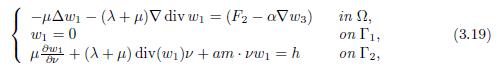
The aim of this work is to prove polynomial decay of enegy for the solutions of the thermoelastic system with second sound and linear boundary dissipation, whose equations correspond to (1.6)-(1.7), (1.5) and:

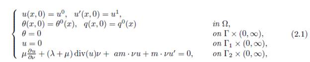
where Γ = Γ₁ ∪ Γ₂, Γ₁ and Γ₂ are defined as

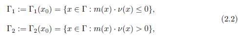
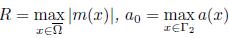
x₀ ∈ ℝ ⁿ, m(x) = x −x₀, and ν(x) = (ν₁(x), · · · , ν_n(x)) is the exterior unit normal vector at Γ at the point x of Γ. The function a = a(x) ≥ 0 satisfies

We also suppose that

where int_Γ is the relative interior of Γ. The following observations can be made from the above conditions:

● The assumptions (2.2) imply that the domain Ω is simply connected and star-shaped with respect to x₀ ∈ Ω. Especially, the domain Ω can be a bounded smooth convex open set.

● Note that in Γ there are no thermal changes, however, at Γ₁ the displacement u is null, this is, the fixed part of the system.

● On the other hand, a dissipation acts in Γ₂ which is linear in the term u^′ and, in particular, describes a displacement in this part of the boundary by virtue of elasticity.

● Since Γ and Γ₁ are closed and Γ₂ the complement Γ₁ in Γ, it follows that so it is not necessary to impose compatibility conditions.

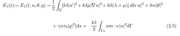
The polynomial decay of energy of solutions is obtained by using the energy method. The definition of the energy E₁(t), known as first-order energy, can be motivated by multiplying (1.6) by kδu^′, (1.7) by kαθ and (1.5) by γαq, and integrating in Ω. The first order energy is defined as follows

satisfying

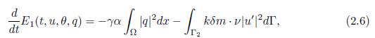
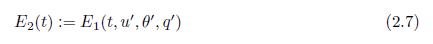
which indicates that the system is dissipative. Analogously, for the second-order energy E₂(t), applying a derivative with respect to t in (1.6), (1.7) and (1.5), multiplying by kδu^′′, kαθ^′, γαq^′ respectively and integrating in Ω , is defined as

with

Now we can state the main result of this work.

Theorem 2.1. Suppose the geometrical conditions (2.2) are valid and

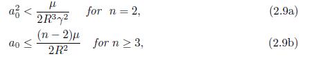
where and a(・) is the function stated in (2.1). Then, for all initial data U₀ ∈ D(Λ), there exists a constant M = M(U₀) > 0 such that the energy of the system (1.6)-(1.7) and (1.5)-(2.1) satisfies

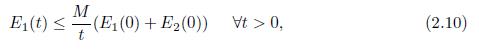
where D(Λ) is defined in (3.7).

Remark 2.2. On the asymptotic study of solutions of differential equations, it is important to note that:

To following section shows the well-posedness of the system.

3. Well-posedness of the system

In order to guarantee the existence and uniqueness of solutions for the system (1.6)-(1.7) with conditions (1.5) and (2.1) the linear semigroups theory will be used. The system can be rewritten as an abstract Cauchy problem for a linear operator and Hilbert space, to be defined later in the paper, mainly by virtue of the linear dissipation at the boundary (2.1). As a tool to obtain the result, we will use the Lumer-Phillips Theorem and consequences arising from this theorem.

Proposition 3.1. Let A be a dissipative linear operator with dense domain D(A) in X. If 0 ∈ ρ(A), with ρ(A) the resolvent set of A, then A is the infinitesimal generator of a C₀ semigroup of contractions on X.

Proposition 3.2. Let (A, D(A)) be the infinitesimal generator of the strongly continuous semigroup (T (t))_t>0. Then, for every x ∈ D(A), the function

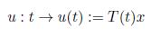
is the unique classical solution of the abstract Cauchy Problem associated to (A, D(A)) and the initial value x

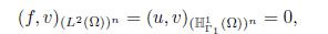
For more details on the theory of linear semigroups and in particular on the proof of this proposition, see for instance [¹², ¹⁴]. In order to define the abstract Cauchy problem associate to System (1.6)-(1.7) one can define the phase space ℍ and the norm induced by the energy of the system as follows. Let ℍ ¹ _Γ1 (Ω) be the space

And

where H¹(Ω) is the usual Sobolev space. Define the norm in (ℍ ¹ _Γ1(Ω))ⁿ as

and the norm in ℍ as

where V = (u, v, θ, q). The following notations will be taken to reformulate the initial value problem (1.6)-(1.7), (1.5)-(2.1) in a first-order system. Let V and V₀ be the vectors

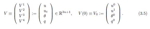
Note that equations (1.6)-(1.7), (1.5)-(2.1) can be written as with

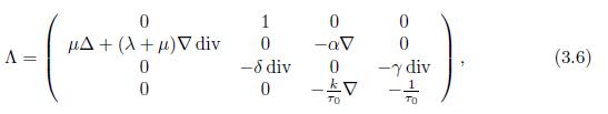
where the domain of Λ is

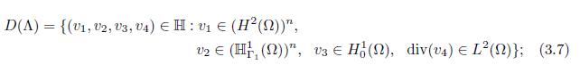
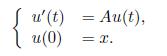
thus, to solve the system (1.6)-(1.7), with conditions (1.5) and (2.1) is equivalent to solve the following abstract Cauchy problem associed to the Λ operator,

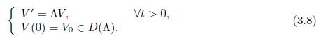
Some properties of the Λ operator are shown in Proposition 3.3.

Proposition 3.3. Let (Λ, D(Λ)) be the operator defined in (3.6) with domain (3.7). Then

As a consequence of this proposition and by the semigroup theory, we have the following result:

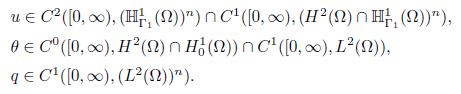
Theorem 3.4. Problem (3.8) has a unique solution V ∈ C ⁰([0, ∞), D(Λ)) ∩C¹([0, ∞), H) given that V (t) = e^−tΛV₀. Consequently, the functions u, θ and q, as the solutions of the system (1.6)-(1.7), (1.5)-(2.1), satisfy

In the proof of proposition 3.3, the regularity estimates described in Theorem 3.4 are outlined. The proof of the proposition 3.3 is proved as follows.

Proof. To prove (a), the following auxiliar set is defined

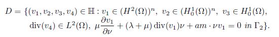
It must be shown that D ⊂ D(Λ) as well as D is dense in H. The inclusion D ⊂ D(Λ) is due to the fact that if (v₁, v₂, v₃, v₄) ∈ D, then v₂ = 0 in Γ, thus

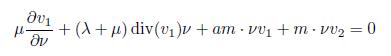
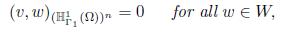
in Γ₂. For density of (C₀ ^∞(Ω))ⁿ and C₀ ^∞(Ω) in (L²(Ω))ⁿ and L²(Ω), it is enough to show the density in (ℍ ¹ _Γ1 (Ω))ⁿ. If W is defined as

then, W is dense in (ℍ ¹ _Γ1 (Ω))ⁿ. In fact, if v ∈ (ℍ ¹ _Γ1 (Ω))ⁿ such that

then for every fixed function f ∈ (L²(Ω))ⁿ, the elliptical problema

has a solution u ∈ W . Thus

showing that v = 0; therefore, W is dense in (ℍ ¹ _Γ1 (Ω))ⁿ due to the Hanh Banach theorem. Thus, the density of D(Λ) in ℍ is proved.

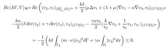
To prove (b), considering the definition of the inner product in ℍ, it is easy to show that Λ is dissipative, since if V ∈ D(Λ) with V = (v₁, v₂, v₃, v₄), then

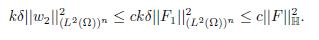
The following proves that −Λ⁻¹ exists and is a continuous operator required to prove (c). Let W be a vector such that W = (w₁, w₂, w₃, w₄) ∈ D(Λ) with ΛW = 0. Then

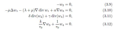
It is clear that w₂ = 0, given that ΛW = 0, then Re(ΛW, W ) = 0; therefore, concluding from (b), w₄ = 0. In addition, from (3.12), ∇w₃ = 0, from (3.7) w₃ ∈ H₀ ¹(Ω), and due to Poincaré’s inequality, w₃ = 0. On the other hand, from (3.10), w₁ would be the solution of the problem

thus, w₁ = 0. Consequently, W = 0 showing that −Λ is an injective operator.

To show that −Λ is a surjective operator, that is, if F = (F₁, · · · , F₄) ∈ H, there exists W ∈ D(Λ) such that ΛW = F , the following system must be solved:

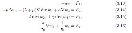
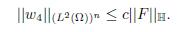
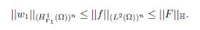
Thus, w₂ ∈ (ℍ ¹ _Γ1 (Ω))ⁿ can be obtained from (3.13) and by using the equivalence of norms (ℍ ¹ _Γ1 (Ω))ⁿ and (ℍ ¹(Ω))ⁿ the following estimation is obtained

From (3.15) is shown that div(w₄) ∈ L²(Ω), from this result and considering (3.16) one gets

As a consequence of the previous expression and the Riesz Theorem, w₃ ∈ H₀ ¹(Ω) is the unique solution of the problem −Δw = g in Ω with g ∈ H⁻¹(Ω). Moreover,

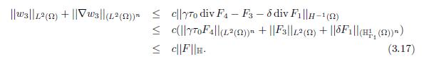
Considering (3.16) and given that w3 ∈ H¹ ₀ (Ω), it holds that w₄ ∈ (L²(Ω))ⁿ. Thus, w₄ satisfies the conditions of the domain D(Λ), that is, w₄ ∈ (L²(Ω))n and div(w₄) ∈ L²(Ω). In addition, from (3.16) and (3.17), one obtains the following estimation

Finally, to prove w1 ∈ (H²(Ω)∩ ℍ ¹ _Γ1 (Ω))ⁿ, it follows the same reasoning as in [10], so we summarize the most important results below.

As w₂ ∈ ℍ ¹ _Γ1 (Ω))ⁿ then if h is defined as

then h ∈ (H^1/2(Γ))ⁿ; and, therefore, w₁ ∈ (ℍ ¹ _Γ1 (Ω))ⁿ is the unique solution of

where f = (F₂ − α∇w₃) ∈ (L²(Ω))ⁿ. In fact, if ϕ ∈ (ℍ ¹ _Γ1 (Ω))ⁿ, then

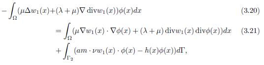
and considering the bilinear application in (ℍ ¹ _Γ1 (Ω))ⁿ × (ℍ ¹ _Γ1 (Ω))ⁿ as

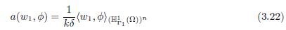
and functional F ∈ [(ℍ ¹ _Γ1 (Ω))ⁿ]′

we have the assumptions of Lax-Milgram Theorem and then there is a unique solution w₁ ∈ (ℍ ¹ _Γ1 (Ω))ⁿ satisfying

In order to prove w₁ ∈ H²(Ω), it is necessary (i) to solve another elliptic problem and, by Nirenberg’s translation method, (ii) to find the regularity in w₁. To do so, it is necessary to apply important results in Sobolev spaces, such as the trace Theorem. In this case, the reasoning and theoretical developments are similar to those obtained in [¹⁰].

4. Stability

This section presents the asymptotic behaviour of the energy of the system (1.6)-(1.7), (1.5) and (2.1), when time t tends to infinity. The aim is to show the result of the polynomial stability of the energy associated with the system by using the multiplier methods of [¹⁰] for the thermoelastic system with boundary dissipations, as well as the ideas discussed in [¹⁷] where a one-dimensional thermoelastic system with second sound is studied. As mentioned in Theorem 2.1, the energy decay to be determined is of the form

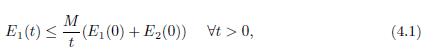
and it depends on the first and second order energies defined in (2.5) and (2.7), respectively. The expression (4.1) will be called polynomial decay of energy.

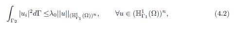
In addition to the constants defined in Theorem 2.1, let λ₀ be denoted as the least positive constant such that

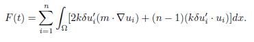
and let F (t) and L(t) be the functionals definied as follows

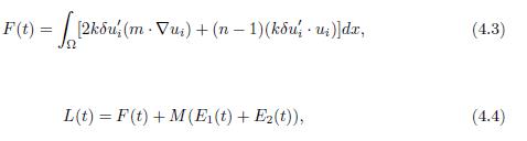
where M > 0 is determined later on. Note that the notation in F (t) simplifies

The proof of Theorem 2.1 is based on the demonstration of a series of properties for the functionals F (t) and L(t). These properties are shown in the following sequence of lemmas.

Lemma 4.1. The functional F(t) satisfies

Proof. Multiplying (1.6) by kδu in (L²(Ω))ⁿ and integrating it in Ω, it holds

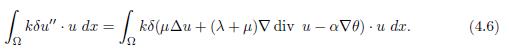
This expression can also be expressed as

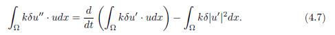
By using Green’s identity and the boundary condition (2.1), the right-side terms in (4.6) have the following expressions

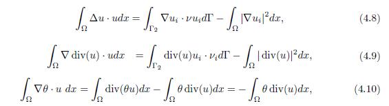
because θ = 0 in Γ. When replacing (4.7)-(4.10) in (4.6), it holds

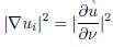
Similarly, multiplying the equation (1.6) by kδm · ∇u in (L²(Ω))ⁿ, given that m · ∇u = (m · ∇u₁, . . . , m · ∇u_n), and integrating it in Ω, it holds

Besides, from the condition (2.1), it holds

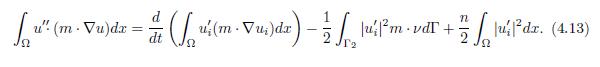
By applying the Green’s identity to the right-side terms in (4.12), and considering the fact that u = 0 in Γ₁ satisfies and , it holds

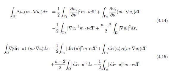
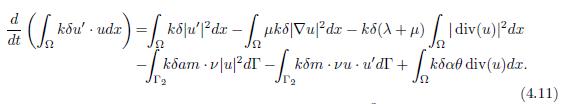
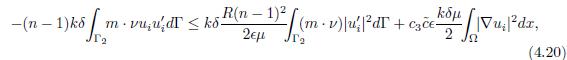
By using condition (1.5) and replacing the results (4.13)-(4.15) in (4.12), one concludes that

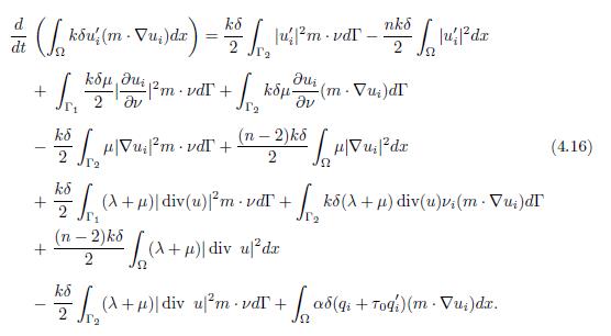
So, from the condition (2.1), and from the expressions (4.11) and (4.16), the functional

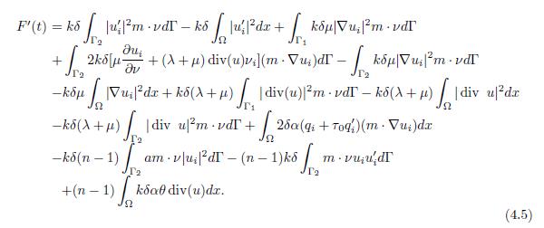
Lemma 4.2. For all ϵ > 0 and under the conditions (1.5) and (2.1), F′ satisfies

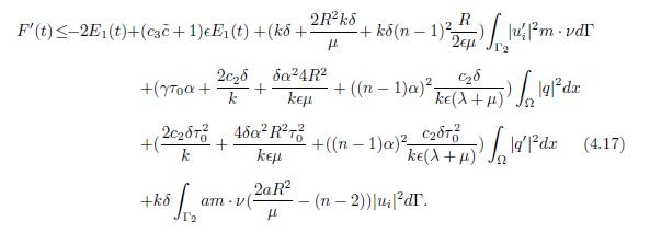
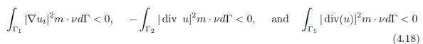
Proof. From the expression (4.5), the following estimates are obtained. First, from the geometric conditions (2.2), the right-side terms in (4.5) satisfy

On the other hand, due to the Poincaré inequality for θ and considering equation (1.5), the following estimation for θ is obtained

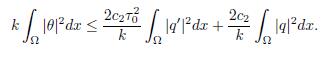
Thus, in (4.5) is estimated as

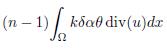
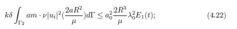
where c₂ is the Poincaré constant. At the same time, due to the Young inequality, the trace Theorem, and Poincaré’s inequality applied to the function u, the following inequalities are obtained:

and

where ĉ is the constant given by the trace Theorem.

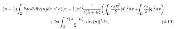
From the Hölder inequality, one finds that

By replacing the expressions (4.18)-(4.21) in (4.5) and adding the terms to complete the energy of first order defined in (2.5), (4.17) is obtained.

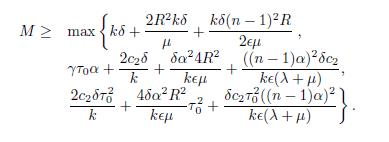
Lemma 4.3. Under the hypothesis of Theorem 2.1, L(t) satifies

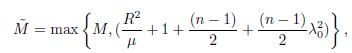
Proof. The proof is given by analyzing the dimension: n = 2 and n ≥ 3. Let M be

In the case n = 2, the function a(x) satisfies (2.9a), then, by using the inequality (4.2), it holds

thus, if ϵ is given by ϵ < 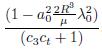then, the case (a) for dimension n = 2 is obtained from Lemma 4.2. Analogously, by using (2.9b) and by taking ϵ < from Lemma 4.2, one can deduce (a) for the case n ≥ 3.

Finally, in order to demonstrate (b) for the Lemma 4.3, one combines the inequality (4.2) and the Cauchy inequality applied to F(t) as shown in (4.3), and defines M as

thus, functional L(t) satisfies (b).

Theorem 2.1 is demonstrated by using the results of the sequence of Lemmas as follows.

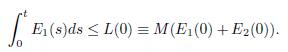
Proof of Theorem 2.1. Given E₁(t) , integrating it on [0, t], and by using the equivalence of Lemma 4.3, one obtains

Moreover, due to

and being , then ; thus

proving the result of Theorem 2.1, and consequently, showing the polynomial decay of the thermoelastic system.