1. Introduction

The operational environment of road vehicles has inflow direction and velocity magnitude that alter continuously. The average natural wind speed on the ground has a value between 2 and 5 km/h on average, yet it differs among regions [¹-³]. When passenger cars, as well as commercial cars, are approached by a side wind, there is an immense increase in the coefficients of resistance. The condition in which the vehicle is more stable is when the geometric center, center of gravity, and stagnation point are in line[¹]. Moreover, in the case of crosswind, the air flowing through the vehicle becomes asymmetric, and it causes the shift of stagnation points towards the direction of the crosswind. As a result, it considerably affects the vehicle’s stability[⁴]. There are basically two classifications of the study related to the wind having asymmetric flow direction to the vehicle (i.e., side wind and crosswind): one is asymmetric flow stability[⁵], and the other is asymmetric flow aerodynamics[⁶] . The latter topic is the focus area of investigation of this work.

Some researchers have investigated the topic related to side wind imposed on vehicles. The side wind effects of high-speed trains were investigated numerically, and afterward, the experiment was conducted, and results were compared. Some angles of wind direction have been imposed on the object. The study found that the yaw angle affects the velocity field distribution in some regions of the object. The aerodynamic coefficients also increased with the increasing value of the yaw angle [⁷]. Another investigation regarding the combination of yaw angle variation and base bleeding has also been studied for a tractor-trailer. When the yaw angle is greater than 3 degrees, a drag reduction is clearly observed. The CFD predicts the effects of bleed rise entrainment flow in the gap of the model and decreases the wake area on the leeward side, and reduces the drag [⁸]. In the case of aerodynamic devise extension, the study of the yaw angle influence on the installation of a tapered rear extension of a vehicle has also been investigated by means of numerical analysis. The smooth extension improved the drag of the vehicle at zero degrees of yaw angle. However, this additional component, together with a kick, successfully reduces the vehicle drag sensitivity at certain yaw angles [⁹]. Different wind angles have also been imposed on a train to examine its aerodynamic behavior. A set of different Reynolds numbers and wind speeds have been implemented to determine the optimal value of wind tunnel tests. The results showed that the pressure coefficient dwindled as the wind angle increased on the leeward side and symmetrical plane of the train [¹⁰].

Moreover, examining the crosswind effect on vehicles demonstrates the more severe conditions that potentially affect a vehicle since the stagnation point extremely shifts towards the wind direction. The shape influence on mean forces imposed on a mini-van type vehicle has been examined [¹¹], which studied the flow around a vehicle under the constant crosswind in a wind tunnel. The result said that a small variation of the A-pillar radius has an essential influence on the side-force and yawing moment. The discussion linked the A-pillar vortex to the change in its intensity at the different velocities of the wind. Some other researchers [¹²] analyzed the influence of the wind barrier on a vehicle. The case investigated in the research was when a vehicle passes in the wake of a bridge tower in crosswind. Then, the response of the vehicle was studied. The results indicated that without a wind barrier, the vehicle response is larger due to increased wind and vehicle velocity, reaching the maximum at 30 degrees of wind direction. The response of side acceleration and yaw angular acceleration was effectively decreased. A comparison of static and moving experiments has also been investigated [¹³] on the stability effects of a model passenger train under crosswind. Pressure distribution on the nose of the model, side, lift, and rolling moment coefficients acting on the model had also been clearly investigated. The study also inferred that static experiments are sufficient in terms of investigating the overall mean aerodynamic side and lift force, and rolling moment coefficient.

The mentioned previous works related to the yawed condition of a vehicle representing side wind and crosswind imposed on a vehicle demonstrate the essential topic of an external aerodynamic of a road vehicle due to asymmetrical wind direction. This work aims to investigate the aerodynamic behavior of a vehicle at a yawed position representing the side wind flowing through the vehicle. The innovation of a vehicle with a water-drop shape becomes a distinctive difference in this work. The study on drag force, lift force, pressure distribution, turbulence kinetic energy, and vortex region are numerically and graphically analyzed under different side wind angles (i.e., the yaw angle of the vehicle). This study will provide a better understanding of the aerodynamic condition of an extremely efficient vehicle with a water-drop shape and assist further research on the external aerodynamics under side wind. Moreover, the study will also contribute to the development of the next vehicle generation not only to the aerodynamic improvement but also to others [¹⁴-¹⁶]. The outcome of this work contributes to the designer, researchers, scholars, and engineers having a better awareness of external aerodynamic behavior due to asymmetrical wind direction imposed on a vehicle.

The picture of the real vehicle and the full-scale model for the simulation are depicted in Figure 1. The so-called extremely efficient vehicle is an electric-powered vehicle with the shape of an external body similar to a water-drop-shaped vehicle from the top view. It consists of three wheels with rear-wheel drive as the drive train and front wheels as the steering control. The inclined position of the driver becomes the most appropriate choice regarding the need for an as-low-as-possible vehicle body. The external body is constructed with carbon-reinforced fiber to make it lightweight and durable. The vehicle competed in the fuel efficiency competition to obtain extremely efficient fuel consumption.

2. Simulation setup

The model for the numerical simulation was constructed with a full-scaled dimension. The total length (L) of the vehicle is 2695 mm, the overall height (h) is 770 mm, and the total width (w) is 850 mm. However, some simplifications had been made in order to simplify the simulation, yet still, maintain the essential detail of the vehicle.

Figure 1 The real vehicle and the dimensions of the vehicle model 

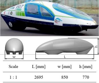
The lower wheel compartment was made as a closed shape with the elimination of the tire that is actually can be seen from the lower part of the vehicle. The presence of a joule meter is actually the main requirement to be placed in the outer part of the real vehicle; yet this component is eliminated in the software simulation since the shape is not really significant in the study’s aims. Some cooling holes in the rear bottom of the vehicle were not considered in the model. The detail of the vehicle model can be observed in Figure 1.

The yawed vehicle model at β = 0 deg, β = 10 deg, β = 20 deg was chosen to simulate the side wind condition. The Y-axis denotes the vertical direction of the vehicle model, and the Z-axis represents the side direction of the vehicle model. The longitudinal direction of the vehicle is constructed at X-axis with -X direction as the wind direction. 50 km/h (13.89 m/s) of vehicle velocity has been chosen by considering the real velocity of the vehicle in all the chosen yaw angles, as depicted in Figure 2.

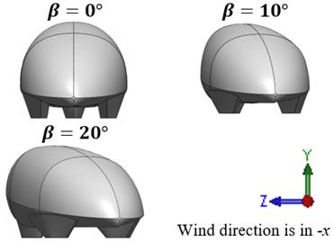
Figure 2 View of vehicle model at yaw angle (β) 0 deg, 10 deg 20 deg to simulate the side winds directions 

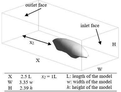
The simulation was performed in a virtual wind tunnel with Ansys Fluent Software Academic Version. This solver has also been employed to investigate a similar problem in aerodynamics [¹⁷-²⁰] , Figure 3 shows the computational domain size of the simulation. The length of the virtual wind tunnel (X) is 2.5, the length of the model (L), the width of the tunnel (W) is 3.35, the width of the model (w), and the height (H) is 2.39 of the height of the model (h). In order to catch the condition of the airflow behind the vehicle model, the distance of the tunnel from the rear part of the vehicle model (x ₂ ) is 1L. These dimensions were chosen considering the limitation of the academic version of the software. However, the chosen dimension was representatively sufficient to capture the reality of the vehicle in real condition since the required investigated location is below the vehicle and the near-rear part of the vehicle.

Figure 3 Computational domain for β = 0 deg 

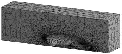
The tetrahedral volume mesh was chosen for the mesh setting. The 1.2 growth rate of element size with a minimum element size of 3.5 mm and a maximum size of 705 mm was chosen as the mesh setting. The mesh quality check was performed with a skewness target of 0.9. The mesh setting uses the medium smoothing and smooth transition of the inflation option. The total nodes are 26,110, and the total elements are 137,219. The resulting mesh has been represented to capture the flow over the vehicle body, as depicted in Figure 4.

The main simulation employs the standard k-ε model with standard wall functions. This turbulence model has been widely employed to investigate external aerodynamic behavior [²¹-²³], However, different turbulence models were applied to compare the results, which will be explained in the next section to validate the results. The fluids were set to air with 1,225 kg/m³ constant density and 1.7894e-05 kg/m-s constant viscosity. The inlet face is the area of the wall in front of the vehicle set with 13.89 m/s (50 km/s) inlet velocity for all the yaw angles with the magnitude normal to the boundary. The outlet face was set to pressure outlet, which is the wall at the rear part of the vehicle opposed to the inlet face, as depicted in Figure 3. The tunnel wall was set to a slip wall since it represents the moving road when the vehicle is running, and the solid wall of the outer vehicle surface was set to a no-slip wall to capture the real condition of the car surface with the standard roughness model.

Figure 4 Section view of the resulted mesh of the model 

3. Results and discussions

3.1 Investigating the main aerodynamic performance

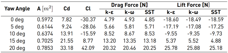
The performances mentioned in this section refer to the projected area, coefficient of drag (Cd), drag force, coefficient of lift (Cl), and lift force. The investigation has been performed by employing different turbulent models to validate the results. The k-ε, k-ω, and SST turbulence model were chosen to calculate the aerodynamic performance at different side wind angles of the vehicle (i.e., different side wind directions) between 0 deg to 20 deg. The projected area increases as the side wind angle is elevated. The amount of area calculated is considered not significant up to 10 deg of side wind angle. The additional area is around 0.02 - 0.03 m². However, after 10 deg of side wind angle, the values of the projected area are far higher than before, which is monitored more than 0.1, and it keeps increasing as the side wind angle elevates. As can be expected from the drag coefficient (Cd) equation as written in Equation (1) at a side wind angle [²⁴]:

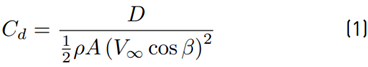
where 𝜌 is the air density, V_∞ is the freestream velocity, A is reference projected area, and β is the yaw angle the increasing value of projected area causes the Cd increment. Another trend to be criticized is the values of the Cl, together with lift forces, are still negative for the side wind angle is 10 deg. It means that the vehicle starts losing the downforce and the grip when the side wind direction is above 10 deg. A similar trend can be observed for the drag force (D) and lift force (L) values at different side wind angles.

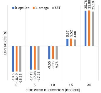
Figure 5 Changes in lift forces at different directions of side wind employing different turbulence model 

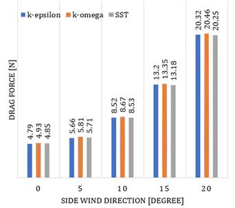
Figure 6 Changes in drag forces at different directions of side wind employing different turbulence model 

The most appropriate turbulence model needs to be selected so that it is able to represent real-world condition [²⁵]. Even if the main turbulence model for this simulation employs k-𝜀 model, it is necessary to compare just in case a different model is employed to verify the results. Three different turbulence models, which are k-ε, k-ω, and SST, were employed to calculate drag force and lift force at different side wind angles of the vehicle in this section. The percentage of deviation among the different turbulence models is less than 3%. It explains that the result for the current turbulence model is representative of capturing the real value of the aerodynamic performance. Table 1 shows the results of this calculation, and Figures 5 and 6 explain the trend of the results.

Table 1 Effects on Aerodynamic Performance 

3.2 Understanding the static pressure distribution and wall shear stress under side wind

The total pressure coefficient is an appropriate visualization to point out where the energy losses are observed in the flow. The pressure coefficient is considered as the non-dimensional ratio between static pressure at the observed point and total pressure of the undisrupted flow, which is defined by Equation (2) as follows [²⁶].

With p is the static pressure at the observed point and p_tot∞ is free stream total pressure.

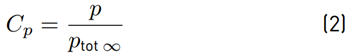
When the airflow is accelerating, the velocity is also getting to increase. It causes the static pressure to decrease and the other way around for decelerating. The losses of energy indicate losses in dynamic or static pressure. Therefore, the total energy losses that are independent of energy form are possible to be investigated with total pressure coefficient visualization. Figure 7 indicates the pressure distribution and the changes in the stagnation point area at the front part of the vehicle at different side wind directions. Figures 8 to 10 show the pressure distribution in terms of pressure coefficient along the vehicle surface. Therefore, it is possible to find the areas responsible for pressure drag. The value of Cp 0, which is the stagnation pressure, starts from the area of the stagnation point due to the side wind direction. The comparison from the Cp results of the vehicle at 0 deg, 10 deg, and 20 deg indicates that the lowest value of the pressure coefficient lies in the area of the tip of the wheel compartment. A considerable increase in the value of Cp occurs. The increasing trend also can be investigated in all other surface areas of the vehicle; however, the trend is not as much as the area of the wheel compartment.

The plot of pressure distribution can also explain the shift of the stagnation point in the fore-end of the vehicle and at the front-below part of the vehicle body surface, as indicated in Figure 7.

Figure 7 Pressure distribution below the front-end of the vehicle at 0 deg, 10 deg, and 20 deg of side wind angles 

Additionally, the skin friction coefficient graphs are plotted in Figures 11 to 13. The skin friction coefficient (Cf) [²⁶] is defined in Equation (3):

Where τ _w is skin shear stress on the vehicle surface [²⁶] which is defined by Equation (4):

With μ is dynamic viscosity, V is airspeed, and y is the distance from the wall.

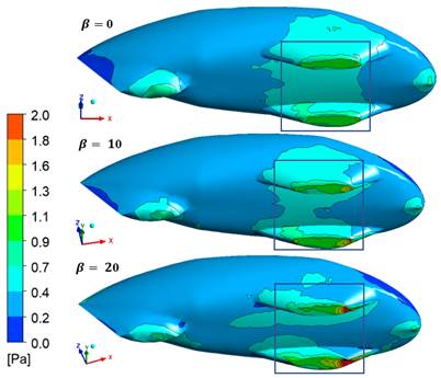
In this case, with the defined air density and the vehicle velocity, the friction coefficient depends merely on the skin or wall shear stress. The wall shear stress indicates the shear stress acting on the vehicle surface resulting from friction between fluid flow and the wall, as represented in the previous equation. Therefore, the wall shear stress occurs on the surface area where the boundary layer of the vehicle surface is present. The location in which the boundary layer is detached indicates the absence (or very low value) of wall shear stress. Eventually, it is possible to observe this phenomenon by observing the Cf plot in Figures 11 to 13. Graphically, the picture of the total wall shear distribution of the vehicle is depicted in Figure 14, Figures 8 to 10 portray the distribution of the pressure coefficient of the vehicle body at different yaw angles. The highest value of the pressure occurs at the area of the front wheel. The higher yaw angle also affects the increment of the value of the pressure coefficient in the body. Moreover, the skin friction coefficient along the vehicle is depicted graphically in Figures 11 to 13. A reverse phenomenon occurs in the value of the skin friction coefficient. While the pressure coefficient goes to a negative value when the yaw angle increase, the skin friction coefficient goes up.

3.3 Analyzing turbulence kinetic energy and vortex region around the vehicle

Turbulence fluctuations naturally have to obtain energy from the main flow. Turbulence kinetic energy is defined as kinetic energy per unit mass of the turbulent fluctuation in a turbulent flow [²⁶]. The energy losses are possibly to be represented in this way. In this section, the investigation focuses on two different planes of the vehicle, which are at the bottom part of the vehicle and the middle part of the vehicle, indicated with Bt and Md, respectively, as it is shown in Figure 15. Figures 16 and 17 show the turbulence kinetic energy at the middle section (Md) of the vehicle and the bottom section (Bt) of the vehicle, respectively.

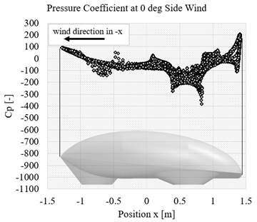
Figure 8 Pressure coefficient at 0 deg of side wind angle along with the position of the vehicle body surface 

The figures visualize the size of the vehicle’s wake at different side wind angles. The vehicle with a zero-yaw angle produces the smallest drag since it generates a noticeably small wake. It means the flow is less disrupted.

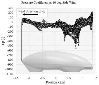
Figure 9 Pressure coefficient at 10 deg of side wind angle along with the position of the vehicle body surface 

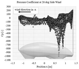
Figure 10 Pressure coefficient at 20 deg of side wind angle along with the position of the vehicle body surface 

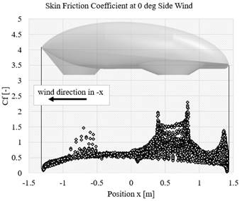
Figure 11 Skin friction coefficient at 0 deg of side wind angle along with the position of the vehicle body surface 

On the other hand, the vehicle with 20 degrees of side wind angle produces a significantly bigger wake as compared to the vehicle with no yaw angle. This region can be observed primarily after the tail of the vehicle on the leeward side.

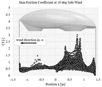
Figure 12 Skin friction coefficient at 10 deg of side wind angle along with the position of the vehicle body surface 

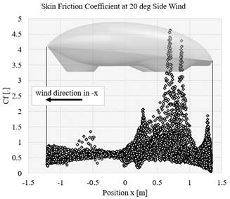
Figure 13 Skin friction coefficient at 20 deg of side wind angle along with the position of the vehicle body surface 

Figure 14 Total wall shear distribution on the vehicle body surfaces at different side wind angles 

The same phenomenon occurs at the bottom side of the plane. The observation indicates the most significant wake region exists on the leeward side of the side wind around the wheel compartment.

Since the drag of the vehicle varies depending mainly on the negative pressure imposed on the vehicle base, the base surface pressure depends on the location in which vortices or recirculation zones in the wake occur. The size of the vortices also contributes to this matter.

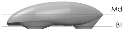
Figure 15 Investigated plane position at the middle (Md) and bottom part around the wheel compartment (Bt) 

Figure 16 Turbulence kinetic energy Bt at different side wind directions 

Figure 17 Turbulence kinetic energy at plane Md at different side wind directions 

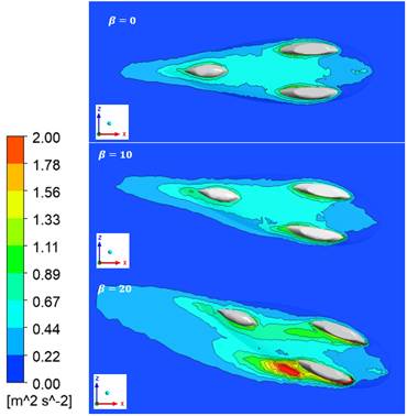
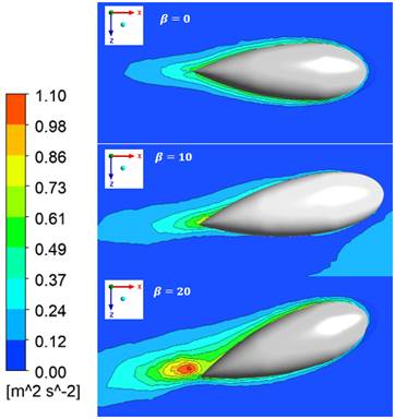
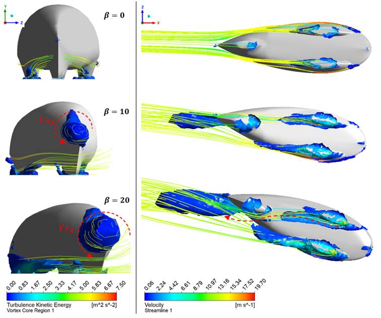
Figure 18 Vortex region showing the generated vortex with its turbulence kinetic energy and the streamlines with its velocity below (right) and the rear part (left) of the vehicle at different side wind directions 

Figure 18 shows the 3D visualization of the vortex region below the vehicle (bottom view) at different side wind directions, together with the velocity streamlines in the vortex region. The vortex region size area is the plot with the absolute helicity method with the actual value of approximately 300 m/s² for all cases to compare the results in different side wind angles easily. The color of vortexes represents the turbulence kinetic energy on it. Together with the streamlines, it is possible to observe the direction of the rotating flow with the velocity of the airflow.

The more the side wind angle is applied to the vehicle, the more it causes a vortex region around the vehicle. The vortex region primarily exists at the lower part around the front wheel compartment and the tail of the vehicle. When the wind flows straightly with respect to the vehicle center point, very less vortex region occurs in every part of the vehicle. However, the increment of side wind direction causes the vortex generation at the wheel compartment and behind the vehicle. Investigating the rearview and at the direction normal to the picture, the streamlines indicate the flow is turning in an anti-clockwise direction when the side wind angle is not equal to zero indicated with Vx _R These vortices get bigger as the increment of side wind angle direction. This phenomenon also has similar results with other works [¹,⁴]. The streamlines from the direction of the wheel compartment seem to be following the direction of the streamlines at the rear part of the vehicle.

4. Conclusions

It can be derived from the previous in-depth explanation that the side wind enormously affects the vehicle’s aerodynamic performance. The values of the coefficient of drag, drag force, coefficient of lift, and lift force exponentially increase if the vehicle imposed on the wind is not symmetrical with the geometrical center and center of gravity. The stagnation point that is depicted in the pressure distribution shifts as the side wind angle increase. The front-wheel compartment becomes the critical location if the investigation is conducted from the point of view of wall shear and pressure coefficient. In terms of the wake region, the more the vehicle yawed, the more vortex region was generated around the wheel compartment and after the vehicle with the considerable circulated flow in an anti-clockwise direction. The dependencies of the drag coefficient, drag force, lift coefficient, and lift force are greatly affected by the direction of the wind. Further work will be carried out on the experimental study considering how the yaw angle affects the aerodynamic coefficient of the vehicle.