English (pdf)
 Article in xml format
 Article references
 Send this article by e-mail
 Cited by SciELO
  Cited by Google
  Similars in
SciELO
Similars in
SciELO  Similars in Google
 Permalink
1. Introduction
Recently, both academia and industry have been interested in implementing the Internet of Things (IoT) technology (commonly used in terrestrial environments) but in underwater environments [1,2]. Some applications proposed using IoT in underwater environments include Submarine pollution monitoring [3], fish farm monitoring [4], climate change monitoring [5], and ocean data collection [6]. Mainly due to costs, wireless communications play an important role in the deployment of these applications. However, underwater wireless communications present new challenges when compared to terrestrial wireless systems. In the literature, it is possible to find some solutions to implement underwater wireless communications: Radio-Frequency communications can also be used in underwater environments, although it is possible to achieve high transmission data rates, the communication range is extremely short [7,8]. Another solution is the use of optical communications [9,10], which has a high transmission data rate but necessarily requires an aligned line of sight, so its use becomes unfeasible in mobile wireless systems. Finally, another solution proposed and widely studied is the use of acoustic modems [11,12], which, although it has a relatively low transmission data rate, has a great communication range and allows total mobility of the transmitter and receiver. Studies that can be found in the literature about acoustic modems include: Location algorithms [13,14], channel estimation [15,16], performance analysis [17,18], and implementation techniques [19,20]. At this point, it is important to note that most of these and other studies [21,22] consider the use of the Orthogonal Frequency Division Multiplexing (OFDM) as the main waveform for transmitting the information. In recent years, new waveforms with better features than OFDM have been proposed and analyzed [23-25]. The new waveform known as Generalized Frequency Division Multiplexing (GFDM) has been considered by many researchers as the most promising, mainly due to the flexibility of this waveform. GFDM is a block-based non-orthogonal multicarrier waveform whose block is composed of M sub-symbols and N sub-carriers which are cyclically filtered by a shaping pulse that is shifted into frequency and time domains [26]. In the literature, it is possible to find several studies about GFDM that include, among others: channel estimation [27], equalization [28], receiver design [29-31], and performance evaluation [32-34]. Even with the considerable advantages of this new waveform, its application in underwater systems has been little explored. A first attempt to analyze the use of GFDM in underwater acoustic communications systems was presented in [35], where mathematical expressions of the power spectral density were derived. This work presents the derivation of general analytical expressions to evaluate the performance of the GFDM waveform operating over underwater acoustic communication channels in terms of the out-of-band emissions and the symbol error probability. The remaining sections of this work are organized as follows. In Section 2, the system model is introduced: mathematical expressions for the GFDM transmitter, the underwater acoustic communication channel, and the GFDM receiver are presented. In Section 3, the development of analytical expressions for the out-of-band emissions and symbol error probability are presented. Using these analytical expressions, numerical results for a particular underwater acoustic communication system are obtained and presented in power spectral density were derived. This work presents the derivation of general analytical expressions to evaluate the performance of the GFDM waveform operating over underwater acoustic communication channels in terms of the out-of-band emissions and the symbol error probability. The remaining sections of this work are organized as follows. In Section 2, the system model is introduced: mathematical expressions for the GFDM transmitter, the underwater acoustic communication channel, and the GFDM receiver are presented. In Section 3, the development of analytical expressions for the out-of-band emissions and symbol error probability are presented. Using these analytical expressions, numerical results for a particular underwater acoustic communication system are obtained and presented in Section 4. Finally, conclusions are drawn in Section 5.
2. System model
2.1 GFDM transmitter
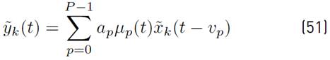
The block diagram of the GFDM transmitter continuous-time model is presented in Figure 1. According to this diagram, the GFDM symbol ˜x k (t) can be expressedas presented in Equation (1) [32].
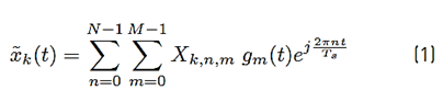
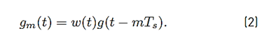
with N denoting the number of sub-carriers, M the number of sub-symbols, and T s the symbol duration. Still in [1], X k,n,m represents the transmitted symbol and g m (t) the transmission filter given by the product of a windowing pulse w(t) of duration T = MT s and a shifted version of a periodic shaping pulse g(t), that is given by Equation (2).
As presented in [32] Equation (3) shows the power spectral density (PSD) of the GFDM symbol defined in Equation (3).
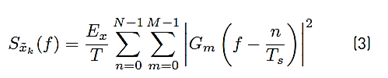
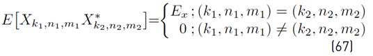
where E x represents the mean energy of the complex symbols X k,n,m , and G m (f) denotes the Fourier transform of g m (t) (see Equation (4)]
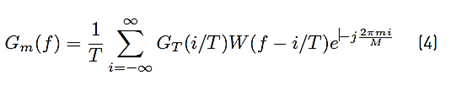
with W(f) denoting the Fourier transform of the windowing pulse w(t) and G T (f) denoting the Fourier transform of one period of the shaping pulse g(t).
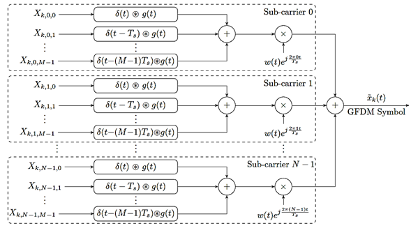
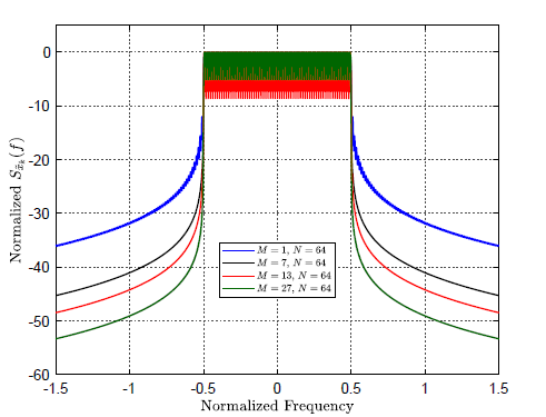
Figure 2 presents the PSD of GFDM symbols for different numbers of sub-symbols. These PSDs were obtained assuming a raised cosine shaping pulse, a rectangular windowing pulse, and using [3] and [4]. This figure shows that the spectral behavior of the transmitted GFDM symbol is improved when high values of M are chosen. Note that when M = 1, the waveform is the classic OFDM.
2.2 Underwater communication channel
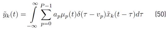
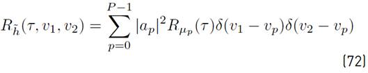
Equation (5), presents the baseband impulse response of the underwater acoustic communication channel that was considered as being a time-varying multipath channel [35-38]
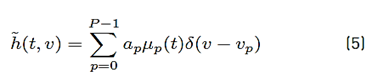
with a p and v p representing the path amplitude and the time-varying path delay, respectively. Still in (5), P represents the number of channel paths, μ p (t) is a complex Gaussian random process with zero mean and δ(·) denotes the impulse function.
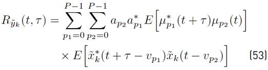
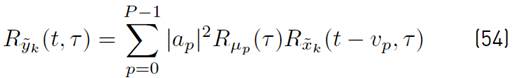
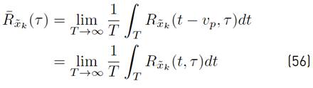
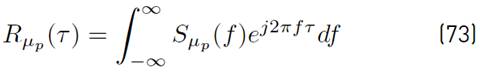
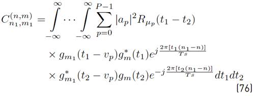
Assuming that complex processes μ p1 (t) and μ p2 (t) are jointly wide-sense stationary and uncorrelated for p1 ≠ p2, Equation (6) presents the autocorrelation function of the underwater acoustic communication channel.
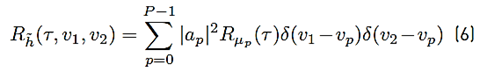
where
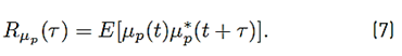
 represents the autocorrelation function of the complex process
 that is, defined by Equation (7).
2.3 GFMD receiver
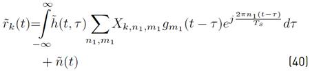
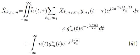
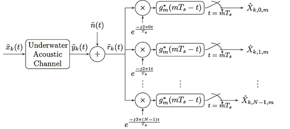
In this work, the GFDM receiver is considered to be a matched filter receiver whose block diagram is presented in Figure 3. Thus, the mathematical expression of the received symbol is presented in Equation (8):
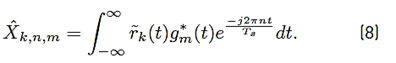
Where
 is given by Equation (9):
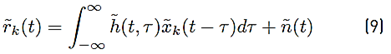
with
 representing the impulse response of the underwater acoustic channel and ñ(t) an additive white Gaussian noise (AWGN) with zero mean and variance N
0.
representing the impulse response of the underwater acoustic channel and ñ(t) an additive white Gaussian noise (AWGN) with zero mean and variance N
0.
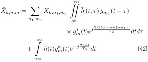
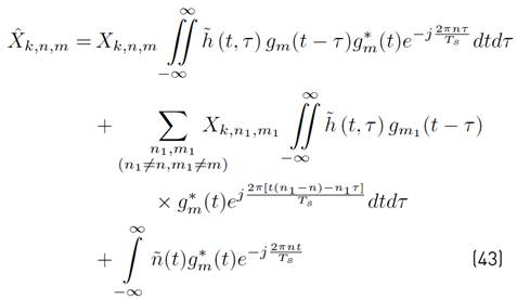
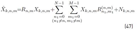
Using [1] in [9], a more compact version of [8] can be written as Equation (10) (See details in Appendix A]:
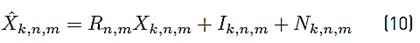
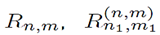
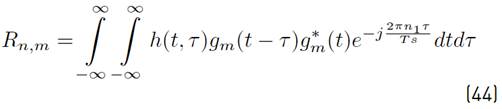
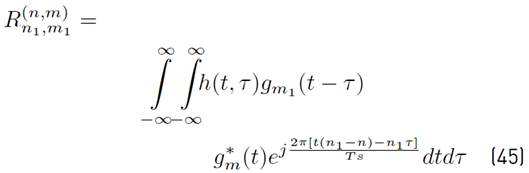
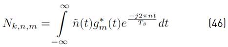
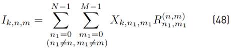
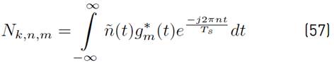
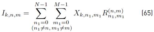
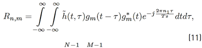
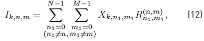
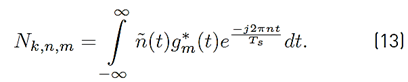
where the mathematical expressions of R n,m, I k,n,m and N k,n,m are presented in Equations (11), (12) and (13) respectively.
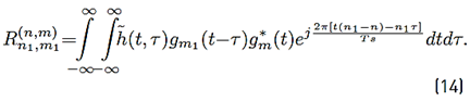
The mathematical expression of
 in (12), is presented in Equation (14).
3. System performance
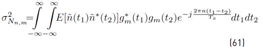
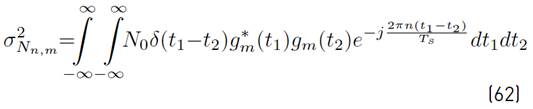
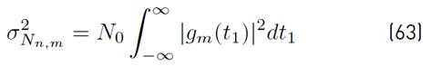
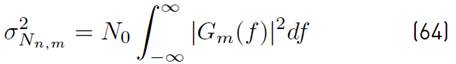
The performance evaluation of GFDM in underwater acoustic communication systems is carried out based on its out-of-band emissions (OOB e ) and symbol error probability. Thus, general analytical expressions of these performance measures are presented below.
3.1 Out-of-band emissions
The received GFDM signal can be expressed as Equation (15):
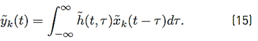
Using [5] in [15] and after some mathematical manipulations,
 can be rewritten as presented in Equation (16).
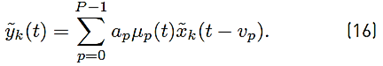
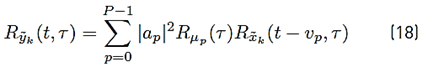
The autocorrelation function of yk(t) defined by (17):

can be expressed as (18):
where
 and
and
 represents the autocorrelation function of
 and,
and,
 respectively.
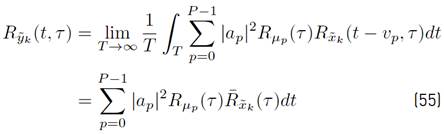
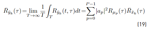
The mean in time of
 is presented in Equation (19) (See details in Appendix B]:
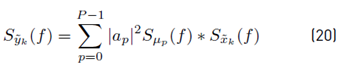
and the PSD of the received GFDM signal is given by the Fourier transform of
 that is, given by Equation (20).
With
 denoting the Fourier transform of
 and
and
 denoting the PSD of the transmitted GFDM symbol defined in [3]. Still in (20), “∗” denotes the convolution operator.
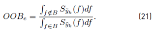
Finally, assuming that the useful bandwidth of the received GFDM symbol is B, Equation (21) shows the OOBe defined as the relationship between the energy outside and inside that useful band.
3.2 Symbol Error Probability
Considering Equation (10), the decision variable, D k,n,m, conditioned to a certain value of R n,m = α, can be written as Equation (22).
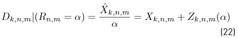
where (23):
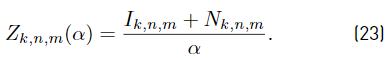
Then, the symbol error probability can be obtained by using Equation (24):
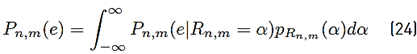
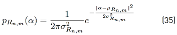
where pR n,m (α) represents the probability density function of R n,m and the conditional error probability of the right side of [24] depends on the digital modulation used. Expressions for this conditional error probability can be found in the literature; for instance, for PSK and QAM digital modulations, these expressions are shown in Equations (25) and (26), respectively [39].
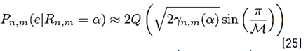
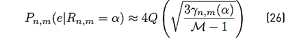
In (25) and (26), M represents the modulation order and γ n,m (α) denotes the symbol energy to noise ratio defined as Equation (27).
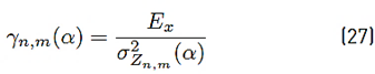
With
 representing the variance of Z
k,n,m
(α). Finally the overall error probability is obtained by using Equation (28):
representing the variance of Z
k,n,m
(α). Finally the overall error probability is obtained by using Equation (28):
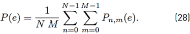
At this point, it is good to note that [25] and [26] are only valid when Z k,n,m (α) is a Gaussian random variable. Results demonstrating this assumption are presented below.
Statistical characterization of Zk, n, m(α)
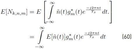
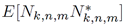
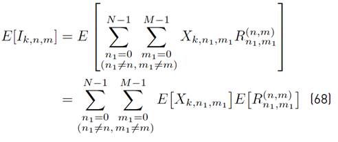
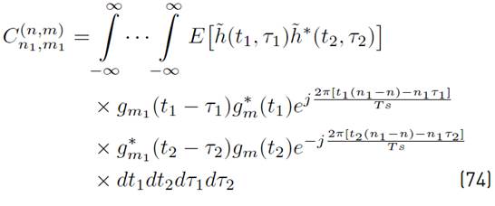
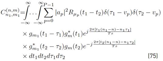
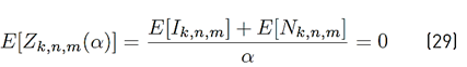
From [12], [13] and taking into consideration the statistical characteristics of the underwater communication channel, h (t, τ), and the AWGN, ñ (t), can be proved that both I k,n,m and N k,n,m not only are Gaussian random variables but also independent of each other. Thus, it is possible to conclude that Z k,n,m (α) is also a Gaussian random variable.
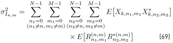
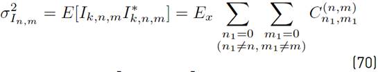
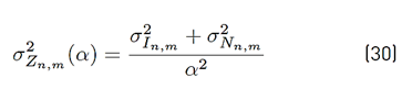
The mean and the variance of Z k,n,m (α) are presented in Equations (29) and (30), respectively.
In (29),
 and
and
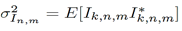
 represents the variance of I
k,n,m
and N
k,n,m,
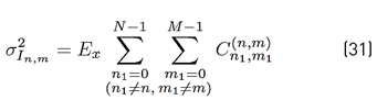
respectively. From [12] is possible to shown that
represents the variance of I
k,n,m
and N
k,n,m,
respectively. From [12] is possible to shown that
 is given by Equation (31).
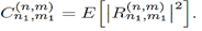
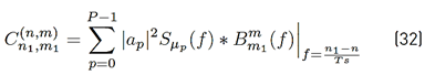
Where (32):
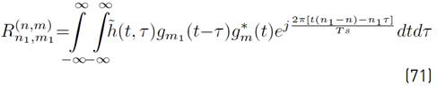
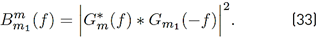
With (33) (refer to Appendix D]:
Analogously, from [13],
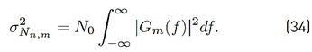
 is given by Equation (34) (referto Appendix C].


4. Numerical results
In this section, numerical results for the OOB
e
and the symbol error probability of GFDM operating over a particular underwater acoustic communication system are presented. The system under consideration uses the BPSK modulation with T
s
= 1μs. In addition, the windowing pulse
 is assumed to be rectangular and the periodic shaping pulse
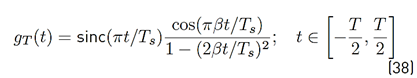
 is a raised cosine with roll-off factor β, meaning that
 is defined as Equation (38).
For the underwater acoustic communication channel, the time-varying multipath model presented in [5] is used with P = 4 and the path delays and amplitudes are assumed to be a
0 = 0.8677, a
1 = 0.4339, a
2 = 0.2169, a
3 = 0.1085, v
0 = 0μs, v
1 = 0.2μs, v
2 = 0.4μs and v
3 = 0.6μs. Still in [5], the random process μ
p
(t) was considered to have Jake’s PSD [40], thereby,
 is given by Equation (39).
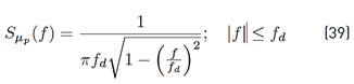
with f d denoting the maximum Doppler shift.
4.1 Spectral evaluation
The PSD of the GFDM received signal
 was obtained only using [3], [20] and [39]. Thus, the OOB
e
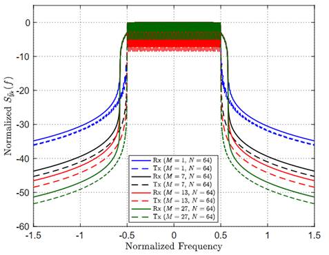
of GFDM operating over the underwater acoustic communication channel was computed using [21]. The effects of the number of sub-carriers and number of sub-symbols over the PSD of the received GFDM signal are shown in Figures 4 and 5, respectively. Here, the considered maximum Doppler shift was 15 Hz. Both figures confirm that the received GFDM signal has lower OOB
e
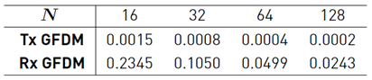
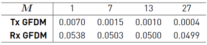
when the N or M values are high. Tables 1 and 2 show the OOB
e
computed values of the transmitted and received GFDM signals for different sub-carrier and sub-symbol values. At this point, it is good to highlight that the PSD of GFDM with M = 1 in Figure 5 also represents the PSD of classic OFDM and, as can be seen in this figure, OFDM has the lowest performance in terms of spectral efficiency.
was obtained only using [3], [20] and [39]. Thus, the OOB
e
of GFDM operating over the underwater acoustic communication channel was computed using [21]. The effects of the number of sub-carriers and number of sub-symbols over the PSD of the received GFDM signal are shown in Figures 4 and 5, respectively. Here, the considered maximum Doppler shift was 15 Hz. Both figures confirm that the received GFDM signal has lower OOB
e
when the N or M values are high. Tables 1 and 2 show the OOB
e
computed values of the transmitted and received GFDM signals for different sub-carrier and sub-symbol values. At this point, it is good to highlight that the PSD of GFDM with M = 1 in Figure 5 also represents the PSD of classic OFDM and, as can be seen in this figure, OFDM has the lowest performance in terms of spectral efficiency.
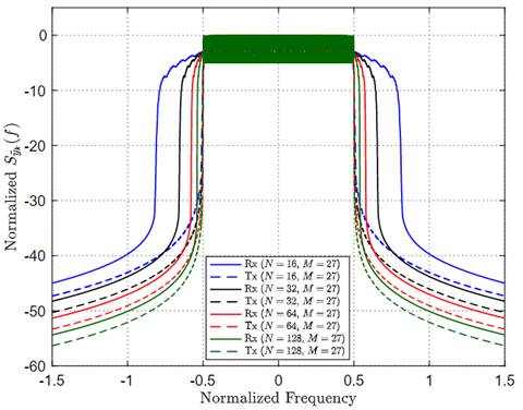
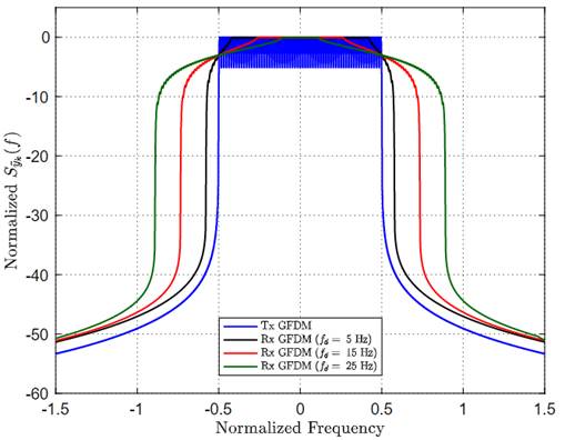
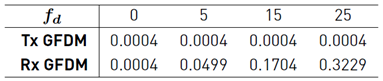
The effect of the maximum Doppler shift typical of the underwater acoustic communication channel is presented in Figure 6. This figure shows the PSD with 64 sub-carriers, 27 sub-symbols, and for different values of f d . In order to make comparisons, this figure also shows the transmitted GFDM signal. Computed values of these OOB e are presented in Table 3. As expected, these results confirm that the lower the maximum Doppler shift, the lower the out-of-band emissions of the system.
4.2 Symbol error probability
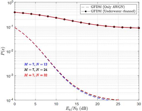
The numerical results of the symbol error probability were obtained using only [24], [25], [27] and [28]. The effects of the GFDM parameters (N, M, α) and the channel parameter f d over the symbol error probability of receiver GFDM are depicted in Figures 7 - 10, respectively. In order to make comparisons, all these figures also show the error probability of the receiver GFDM corrupted only by AWGN. These figures reveal that the presence of a time-varying channel (underwater acoustic communication channel) seriously degrades the symbol error probability of the system.
Figure 7 shows the symbol error probability for an underwater system with different values of N. The other parameters of the system, this is, the number of sub-symbol, the roll-off factor and the maximum Doppler shift, were set to be 7, 0.5 and 10 Hz, respectively. As can be seen in this figure, the symbol error probability is weakly dependent on the number of sub-carriers for both, systems operating over an underwater acoustic channel and systems only corrupted by AWGN.
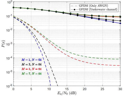
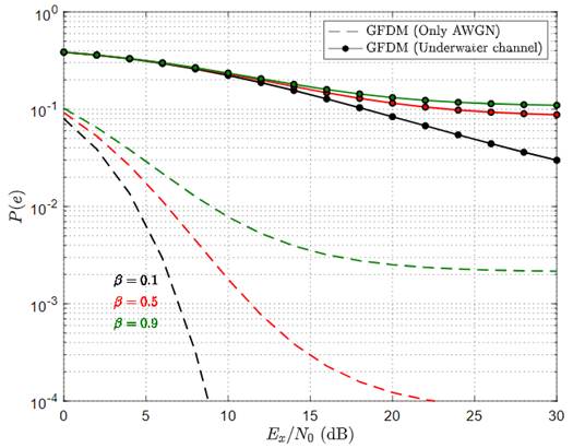
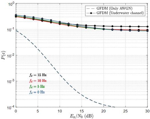
The symbol error probability for an underwater system with different values of M is presented in Figure 8. Here, the number of sub-carriers, the roll-off factor and the maximum Doppler shift were set to be 64, 0.5 and 10 Hz, respectively. This figure reveals that symbol error probability is strongly dependent on the total number of sub-symbols. As expected, while considering high values of M, the symbol error probability is also high. As mentioned before, the GFDM with M = 1 represents the classical OFDM, which in terms of symbol error probability, has the best performance. Figure 9 resents the effects of the roll-off factor α on the symbol error rate probability of an underwater system. This time the number of sub-carriers, number of sub-symbols and maximum Doppler shift were set to be 64, 7 and 10 Hz, respectively. This figure confirms that symbol error probability is strongly dependent on the excess bandwidth of the periodic shaping pulse g(t). Considering low values of excess bandwidth results in low error probability values. Finally, the effects of the maximum Doppler shift on the symbol error probability are presented in Figure 9. The curves presented in this figure were obtained considering 64 sub-carriers, 7 sub-symbols and β = 0.5. From this figure, it is clear that the mobility of the receiver seriously degrades the error probability of the system.
5. Conclusions
The most important contribution of this work is the derivation of analytical expressions of the symbol error probability and out-of-band emissions from underwater acoustic communications systems using the GFDM. The methodology used to obtain these analytical expressions was described in detail in Section 3. As shown in the numerical results, these expressions can easily provide curves for the power spectral density and the symbols error probability with different system parameters. The numerical results obtained show that the number of sub-symbols, number of sub-carriers, and the roll-off factor of the formatting pulse play an important role in the performance of the system, both in terms of spectral efficiency and error probability. These results also reveal that, when a matched filter receiver is used, distortions induced by underwater channels not only degrades the spectral performance of the system (e.g., increase out-of-band emissions) but also seriously increase the symbol error probability; thus, further studies on more complex receivers should be performed.