Artículo de investigación/Research article

A comparison of robust Kalman filtering methods for artifact correction in heart rate variability analysis

Comparación de métodos de filtro de Kalman robustos para corrección de artefactos en el análisis de la variabilidad de la frecuencia cardiaca

Carlos D. Zuluaga-Ríos¹, Mauricio A. Álvarez-López², Álvaro A. Orozco-Gutiérrez³

¹Magíster en Ingeniería Eléctrica, Programa de Ingeniería Eléctrica, Universidad Tecnológica de Pereira, Pereira-Colombia, cardazu@utp.edu.co

²Ph.D. en Ciencias de la Computación, profesor asociado del Programa de Ingeniería Eléctrica, Universidad Tecnológica de Pereira, Pereira-Colombia, malvarez@utp.edu.co

³Ph.D. en Bioingeniería, profesor titular del Programa de Ingeniería Eléctrica, Universidad Tecnológica de Pereira, Pereira-Colombia, aaog@utp.edu.co

Fecha de recepción: 23 de mayo de 2014 / Fecha de aceptación: 18 de julio de 2014

Como citar / How to cite

C. D. Zuluaga-Ríos, M. A. Álvarez-López y A. A. Orozco-Gutiérrez, “A comparison of robust Kalman filtering methods for artifact correction in heart rate variability analysis”, Tecno Lógicas, vol. 18, no. 34, pp. 25-35, 2015.

Abstract

Heart rate variability (HRV) has received considerable attention for many years, since it provides a quantitative marker for examining the sinus rhythm modulated by the autonomic nervous system (ANS). The ANS plays an important role in clinical and physiological fields. HRV analysis can be performed by computing several time and frequency domain measurements. However, the computation of such measurements can be affected by the presence of artifacts or ectopic beats in the electrocardiogram (ECG) recording. This is particularly true for ECG recordings from Holter monitors. The aim of this work was to study the performance of several robust Kalman filters for artifact correction in Inter-beat (RR) interval time series. For our experiments, two data sets were used: the first data set included 10 RR interval time series from a realistic RR interval time series generator. The second database contains 10 sets of RR interval series from five healthy patients and five patients suffering from congestive heart failure. The standard deviation of the RR interval was computed over the filtered signals. Results were compared with a state of the art processing software, showing similar values and behavior. In addition, the proposed methods offer satisfactory results in contrast to standard Kalman filtering.

Keywords: Artifact correction, electrocardiogram, heart rate variability, inter-beat interval, robust Kalman filtering.

Resumen

La variabilidad de la frecuencia cardiaca (HRV) ha recibido una atención considerable por mucho años, ya que esta proporciona un valor cuantitativo para examinar el ritmo sinusal modulado para el sistema nervioso autónomo (SNA). El SNA juega un papel importante en campos clínicos y fisiológicos. El análisis de la HRV se puede realizar calculando varias medidas tanto en el domino del tiempo como en la frecuencia. Sin embargo, el cálculo de estas medidas se puede ver afectado por la presencia de artefactos o latidos ectópicos en registros de electrocardiogramas (ECG). Esto es particularmente cierto para registros ECG desde un monitor Holter. El objetivo de este trabajo fue estudiar el rendimiento de varios filtros de Kalman robustos para la corrección de artefactos. Para nuestros experimentos, se usaron dos bases de datos reales: el primer conjunto de datos incluye 10 series de tiempo de intervalos RR a partir de un generador de series de tiempo de intervalos RR realista. La segunda base de datos contiene 10 conjuntos de series de intervalos RR de cinco pacientes sanos y cinco pacientes que sufren una insuficiencia cardiaca congestiva. Se calculó la desviación estándar de los intervalos RR a partir de las señales filtradas. Los resultados se compararon con un reconocido software de procesamiento, mostrando comportamientos y valores similares. Adicionalmente, los métodos propuestos ofrecen resultados satisfactorios en comparación con el filtro de Kalman estándar.

Palabras clave: Corrección de artefactos, electrocardiograma, variabilidad de la frecuencia cardiaca, intervalos entre latidos, filtros de Kalman robustos.

1. Introduction

The autonomic nervous system (ANS) plays an important role in clinical and physiological fields; but it also is present in several pathological disorders such as diabetic neuropathy, myocardial infarction and congestive heart failure (CHF) [1]. The ANS is divided into three main sub-systems: the enteric, sympathetic and parasympathetic systems. These sub-systems aid to control the internal organs of the body. The autonomic status of these sub-systems on the heart may be indicated and measured by heart rate variability (HRV) [2]. HRV is a noninvasive method to evaluate and analysis cardiovascular diseases such as CHF, coronary heart disease and diabetic neuropathy [3].

HRV has received considerable attention for many years, since it is a quantitative marker for examining the sinus rhythm modulated by the ANS. HRV is the term that defines the variation in heart beat interval (RR interval). To perform HRV analysis it is necessary to obtain an ECG recording from the patient. The RR interval time series can be extracted from these recordings. In the literature, there are three possible forms to measure the HRV: time domain methods, frequency domain methods, and non-linear methods [4].

For diagnosis, several HRV measurements can be computed [4], one of them is the standard deviation of the RR interval (SDRR), that reflects overall variations within the RR interval series, that is, in patients with congestive heart failure, is possible to obtain lower SDRR values in comparison to healthy patients [5]; besides SDRR is sensitive to artifacts [6]. Such measurements are important for representing quantitatively the HRV, but its analysis can be interfered by artifacts, leading to a bias in the HRV measures [7]. Artifacts can produce abrupt oscillations from the mean in the RR interval time series, a behavior that it is not expected to occur in practice. Therefore, the preprocessing or the artifact correction stage is essential in clinical Holter reports for obtaining measurements with excellent quality.

Different methods have been proposed for artifact removing in RR interval time series, including nonlinear predictive interpolation [7], integral pulse frequency modulation [8], and impulse rejection filters [9]. These methods are widely used to reduce the effects of outliers; however, these techniques assume the stationarity of the time series cannot identify anomalous intervals and work in off-line mode.

In this paper, we applied three robust Kalman filters to estimate an RR interval time series. The weighted robust Kalman filter (wrKF) proposed in [10], the robust statistics Kalman filter (rsKF) proposed in [11] and the thresholded Kalman filter (tKF) proposed in [10] and [12]. The first two methods use a weighted recursive approach, where each weight can be considered as the probability of the observed value not being an artifact. The tKF employs a comparative criterion computed for each observation. If the value of the criterion is below a certain threshold, the observation is discarded.

Our purpose was to obtain HRV measurements derived from the robust filtered signals, and compare those values to the ones obtained by cubic splines interpolation, that is a method that replaces missing interbeat interval, included in state of the art clinical software. Several references use this clinical software for approving or comparing their theories [13], [14]. The contribution of our study is the presentation and use of robust methods for artifact correction, which are recursive approaches and they can be applied to stationary and non-stationary environments.

Experimental results obtained include the application of the different methods described above over a real data set and artificial data. The real data set was obtained from MIT-BIH normal sinus rhythm RR interval database and the BIDMC congestive heart failure database (MIT-BIH BIDMC database) [15]. The recordings for first database provide a set of 5 RR-interval time series of healthy patients and 5 patients suffering from congestive heart failure (CHF) [15]. The second data set are artificial data from a realistic RR interval generator proposed by McSharry and Clifford in [16]. These simulated data were compared and validated using real data from MIT-BIH normal sinus rhythm RR interval database, showing consistent results according to the literature, for more details see [16].

The paper is organized as follows. Section 2 presents the material and methods that were used for performing artifact correction based on robust Kalman filtering in RR interval time series. In section 3, we present and discuss the results obtained when applying the methods mentioned before. Finally, conclusions are described in section 4.

2. Materials and methods

2.1 Datasets

For our experiment, we used a realistic RR interval generator proposed in [16]; and the MIT-BIH BIDMC database, which are managed by PhysioNet [15]. Each time series in the databases is about 24 hours long (approximately 100000 intervals). The first data include 10 artificial RR interval time series that simulate temporal and spectral RR intervals during periods of sleep and wakefulness of healthy patients. These simulated data were compared with real data from MIT-BIH normal sinus rhythm RR interval database, showing that real and artificial data present similar results, for more details see [16]. The second dataset provides a group of 5 RR-interval time series from healthy patients and 5 patients suffering from congestive heart failure (CHF). The dataset contains healthy patient’s recordings, with ages ranging from 20 to 45 years old, and from both genders; on the other hand, non-healthy patients’ ages range from 48 to 71 years old, and they include only male. All of the time series were obtained from continuous ambulatory (Holter) electrocardiograms (ECGs). Additionally, artifacts can exist due to missed or false inter-beat detections in the recordings.

2.2 Kalman filter

An algorithm that provides excellent characteristics of state-prediction into a recursive structure approach under several conditions is the Kalman filter. In addition, it only employs the current observations from the data for performing the prediction. It is possible to apply the Kalman filter to stationary and non-stationary environments [17]. The Kalman filter efficiently performs state-inference in a linear dynamical system represented in a state-space form. It is supported in the following relationships.

where {z_k}^N_k=1 are observations over N time steps, {x_k}^N_k=1 are the corresponding hidden states (where x_k ∈ ℝ^{n x 1} and z_k ∈ ℝ^{m x 1}), C_k ∈ ℝ^{m x n} is the observation matrix, A_k ∈ ℝ^{n x n} is the state transition matrix, w_k ∈ ℝ^{n x 1} is the state noise at time step k, and v_k ∈ ℝ^{m x 1} is the observation noise at time step k. It also assumes that w_k and v_k are both uncorrelated additive mean-zero Gaussian noises, this is, w_k~(0, Q), v_k~𝒩(0, R), where Q ∈ ℝ^{n x n} and R ∈ ℝ^{m x m}. Q and R are both diagonal covariance matrices for the state and observation noise, respectively. Hereafter, matrices A_k, C_k, Q and R are jointly denoted as θ = {A_k   C_k   Q   R}.

With knowledge of the Kalman filter parameters (θ), the expected value of the hidden states can be computed by maximizing the likelihood between the state vector x_k and the observation z_k at time k, given the observations until time k - 1, and the parameters θ, p(x_k, y_k |y^k-1₁, θ). This maximization is equivalent to minimize the negative logarithm of the likelihood, leading to the following minimization problem,

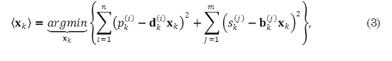
where ⟨ ⟩ denotes the expectation operator; n is the number of states; m is the number of outputs; x_k^- and Σ_k^- denotes the prior estimate of x_k and the prior covariance matrix of the estimation error, respectively. p_k⁽ⁱ⁾ are the entries of the vector 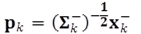s_k^(j) are the entries of the vector 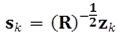; d_k⁽ⁱ⁾ are the entries of the matrix ; and b_k^(j) are the entries of the vector .

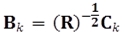Consequently, the expected value for x_k, can be obtained using

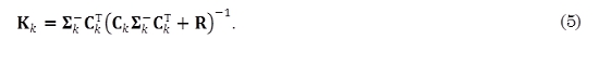
where ⟨x_k⟩ is the posterior estimate of the state vector x_k. Matrix K_k usually known as the Kalman gain, and it is given as

2.3 Robust Kalman filter

In this section, we describe the different methods for robust Kalman filtering that were implemented for estimating the RR interval. In the literature, different ways have been shown for improving the performance of standard Kalman filter (sKF) in presence of artifacts or outliers, but the parameter estimation approaches, for these improvements, are complicated for dynamical systems [10].

2.4 Weighted robust Kalman filter

In [10], Ting et al. proposed a weighted least squares approach that assigns weights w_k to each observation z_k. These weights are random variables that follow a Gamma distribution, that is, 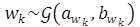, where is the Gamma distribution with parameters a_wk and b_wk.

The difference between this model and the sKF model is the inclusion of the scalar weight wk in the conditional probability of the observation z_k given the state x_k.

For the weighted robust Kalman filter (wrKF), inference over the state vector x_k also operates by applying (4), and Kalman gain matrix is computed as,

Notice the influence of the weights w_k over the Kalman gain K_k. The values for θ and w_k, in (6), can be computed through a variational EM algorithm [18], proposed in [10].

2.5 Robust statistics Kalman filter

In a similar way to the wrKF, in [11], Cipra and Romera introduce a weight vector for each observation, based on the theory of maximum likelihood estimation for robust statistics discussed in [19]; a robust estimate for the state vector x_k can be obtained by minimizing (7) [11],

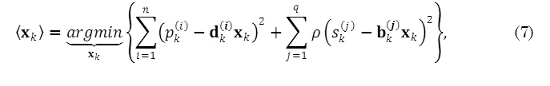
where p(·) is a loss function given as [19]

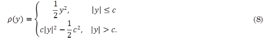
The constant c is chosen according to the degree of loss penalization. Notice that in the sKF model, the loss function p(·) in (3) is equal to the identity function.

For the Robust statistics Kalman filter (rsKF), it can be shown [11] that the Kalman gain matrix is given as

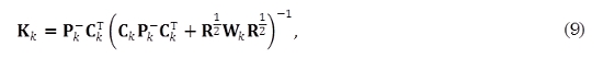
where W_k = diag {w_k⁽¹⁾, ..., w_k^(q)}. Weights {w_k^(j)}^q_j=1 at time k are computed using (10)

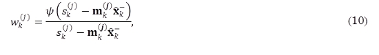
where ψ(·) is the Huber’s loss function,

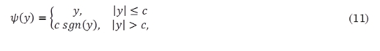
where sgn(·) is the sign function. For our experiments the value of c, in (11), was set as c = 1,645 for a 5% contamination of the data [11].

For applying the rsKF, we use the same equations used for the sKF, except for the Kalman gain matrix, see (5), that takes the form that appears in (9).

2.6 Thresholded Kalman filter

The thresholded Kalman filter (tKF) determines that an observation is an artifact if the residual error between the observation, z_k, and the predicted observation, C_kx_k^-, has a value higher that a predefined threshold. Let us define the residual error as γ_k = z_k - C_kx_k^-. It can be shown [10] that the covariance for the residual error k is computed by using S_k^- = (C_kΣ_k^-C_k^T + R_k)^-1 where the values for C_k and R_k are computed using the same form used for the rwKF. For each observation z_k, the following condition is evaluated

where β is a positive threshold, manually tuned for each data set. The quantity γ_k^TS_k^-γ_k is known as the Mahalanobis distance. If the Mahalanobis distance for γk is greater than β, the observation z_k is assumed to be affected by artifacts and hence discarded. In this case, the posterior estimate state vector ⟨x_k⟩ is assigned to be the prior estimate of the state vector x_k^-.

2.7 Validation

To validate the HRV analysis and compare the performance of the methods, SDRR has been computed, given by [4]

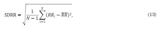
where RR_i is the value of i-th RR interval, N is the total number of successive intervals and RR is the mean value of RR intervals values. The SDRR can be used as a measurement of the short-term variability; this measurement is given in millisecond (ms).

With the aim to study if there are differences that are statistically significant for the results obtained by all filters, using the artificial data, we apply a Lilliefors test form normality over the 10 RR interval time series from the realistic RR interval generator. If the null hypothesis for normality is rejected, we perform a Kruskall-Wallis test to compare average performances among the methods. If null hypothesis for equal medians is rejected, we perform a multiple comparison test using Tukey-Kramer to study further which methods are different. All the significance levels are measured at 5%.

Finally, the Fisher criterion is computed for healthy and CHF patients of MIT-BIH BIDMC database, using SDRR metric. This criterion is defined as follows [18],

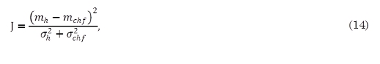
where m_h and σ²_h re the mean and variance of SDRR for the healthy patients respectively; m_chf and σ²_chf are the mean and variance of SDRR metric for the CHF patients.

3. Results and discussion

The wrKF, rsKF, tKF and sKF were evaluated and compared over the data sets described in materials and methods section. The advanced HRV analysis software, Kubios HRV (version 2.1) [20], developed at the Biosignal Analysis and Medical Imaging Group, Department of Applied Physics, University of Eastern Finland, has been used as a baseline to compare the values found for each method of the above methods for the SDRR. For all the filters and the sake of simplicity, one state was used (n = 1, see (1)), and one output was observed (m = 1, see (2)). For the wrKF and tKF, the parameters θ were computed through a variational EM algorithm [18]. The parameter β in (12) was manually tuned to 2. On the other hand, the parameters θ for the rsKF and sKF, were assumed as A = C = I and Q = R = 10^-4 I [10]. To apply Kubios HRV, we used a very strong level for the artifact correction configuration. The Kubios employs a suitable interpolation method for reducing this artifact [20].

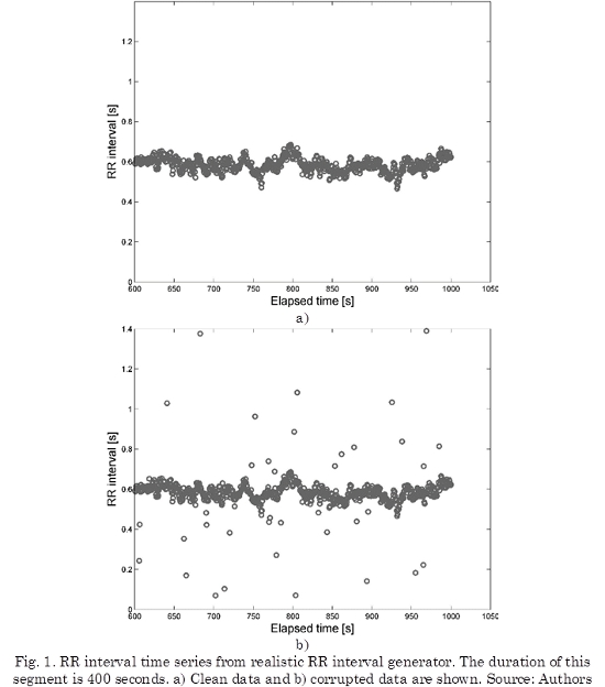
With the aim of observing the robustness of filters, outliers were introduced randomly. Fig. 1a shows an example of the artificial RR interval time series, Fig. 1b shows the same time series corrupted by outliers (Outliers corresponds to 5% of data).

We have applied the filters to the entire artificial data, but for visualizing, we have shown 400 seconds of the time series, as can be seen in Fig. 2.

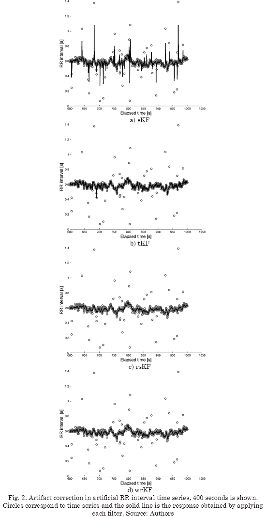
The SDRR, see (13), was computed using artificial data set for each filter. From Table 1, clean data obtained a SDRR of 21.1181 ± 1.2635 ms, and the sKF obtained the highest SDRR value of 54.0252 ± 16.382 ms. This value is due to the influence of artifacts on the predictions.

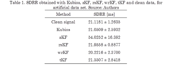
The SDRR calculated for the Kubios is 21.0509 ± 2.5932 ms, the remaining filters obtained values close to the Kubios value. From this table, we can mention that the tKF value was the closest to the Kubios. According to the statistical tests, we notice that the mean rank of SDRR obtained by sKF is significantly different in comparison with the values employing the clean signal, Kubios, wrKF and tKF. The test analysis also shows that there are not methods with mean ranks significantly different for the rsKF values, although of SDRR value for rsKF, in Table 1, presents minor variability and it is close to the clean data value.

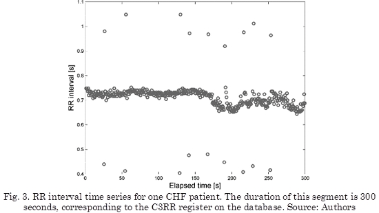
On the other hand, RR interval for one of the CHF patients from MIT-BIH BIDMC database is shown in Fig. 3. This time series corresponds to the C3RR register on the database. This register corresponds to a 48-years old male. For visual reasons, 300 seconds of the register are only shown in Fig. 3.

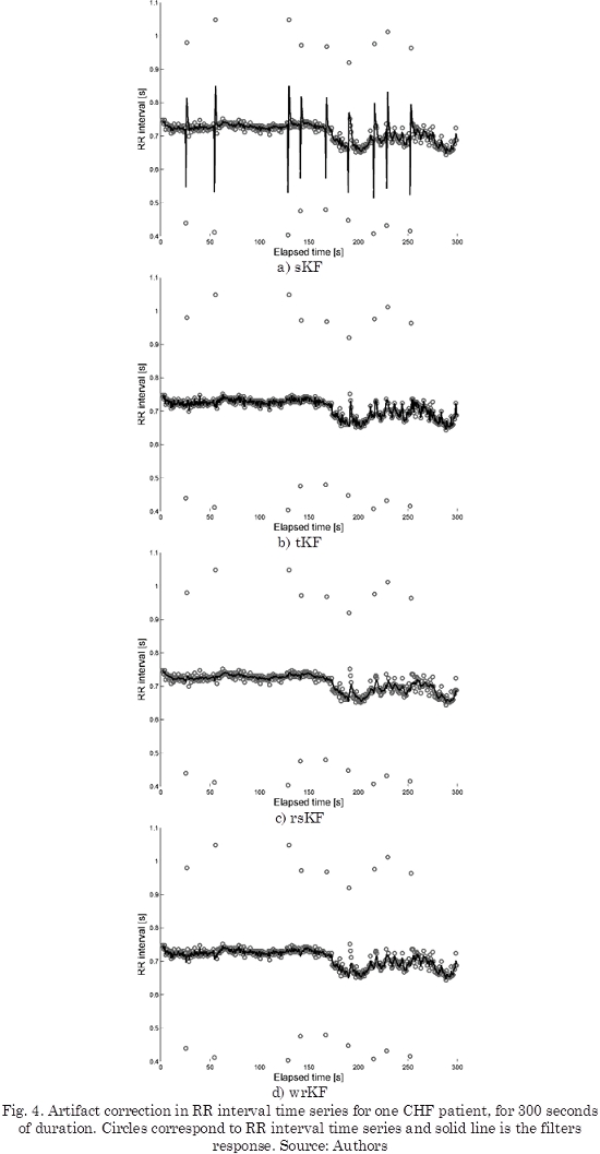
The results of performing the artifact correction with tKF, rsKF and wrKF are shown in Fig. 4b, 4c and 4d, respectively. It is important to notice that all filters were put into use for all length of the data, but only 300 seconds of the registers have been shown.

SDRR is shown in Table 2. We notice reduced values for these measurements for CHF patients in comparison with healthy patients, that is, CHF patients present a reduction in dynamic complexity. The mean of the SDRRs for the healthy patients in this study are between 28.8637 ± 3.8338 ms and 30.2063 ± 4.7041 ms, while the obtained values for the CHF patients are between 8.5433 ± 2.4169 ms and 13.396 ± 2.3392 ms. In [5] was proposed a scheme of preprocessing RR interval time series for HRV analysis, obtaining results consistent with ours.

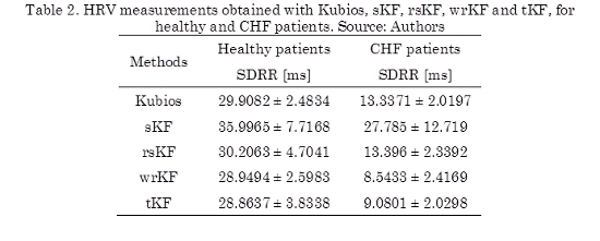
We also notice that differences between healthy metrics and CHF metrics, result very similar for all methods. The sKF presents inaccurate values for these metrics, since it is sensitive to artifacts or outliers present in RR interval series (see Fig. 4a). For example, the obtained results for the CHF patients, in Table 2, show that the sKF computed a SDRR of 27.785 ± 12.719 ms, which is similar to the value found by Kubios in healthy patients (29.9082 ± 2.4834 ms).

It can also be seen from Table 2, that the results obtained from the processing software are very much alike with the rsKF results.

With respect to the wrKF and tKF, the predictions obtained for both methods were more weighted and rejected, respectively, than rsKF. Both methods presented minor differences when compared to the Kubios measurements.

Hence, the robust Kalman filters follow the same behavior compared with this software; and they are suitable tools for artifact correction, considering to the MIT-BIH BIDMC database. We notice that the rsKF achieved the best results, since if we observe the difference between the obtained values from each filter and the processing software values, rsKF achieved the lowest difference values, as shown in Table 2. From the statistical tests, we notice that for Healthy patients, the methods do not have mean ranks significantly different, since their values are closer to each other. For CHF patients, we notice that the mean rank of SDRR obtained by sKF is significantly different in comparison to the values employing the Kubios, rsKF, wrKF and tKF, respectively.

From obtained results of SDRR in Table 2, using Kubios, sKF, rsKF, wrKF and tKF, the Fisher criterion (J) (14) is calculated for all proposed methodologies, as can be seen in Table 3. The idea of using J is to find a value of the function that measures the separation between the SDRR metric for Healthy patients and the metric for CHF patients, while this separation is large, state of the patients is possible to be recognized more easily, therefore, artifact correction methods are adequate.

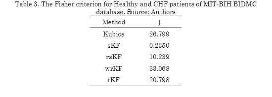
Since achieved results for sKF of SDRR in Table 2, are confused, because this metric for both patients are similar. This is also to see in Table 3, J is calculated for sKF and presents the lowest value in the table, showing the state of the patient can not recognize.

Kubios obtained a criterion of 26.799, and the robust filters also present values greater than sKF values, but rsKF due to the weighting of the predictions obtains a low criterion of 10.239. From this table, it is possible to notice, that wrKF achieved the highest Fisher criterion value (33.068), it shows that the cluster of RR interval series from healthy and CHF patients, using wrKF can be more compact and separated that the others methodologies, however, the Fisher criterion value obtained by Kubios and tKF are close to the Fisher criterion value employing wrKF.

4. Conclusiones

In summary, we have presented three robust Kalman filters for estimating RR interval time series, with the aim of artifact correction. A comparative analysis was performed, it presented similar values with respect to a Kubios; from this study, the sKF is not a good choice for artifact correction, it presents bias in the HRV measures; on the other hand, the robust filters showed to have similar values for SDRR, in comparison with advanced tools. tKF and wrKF rejected and weighted, respectively, too much the predictions, presenting reductions in the HRV metric in comparison with Kubios. Finally rsKF showed to be an appropriate choice for robust filtering in RR interval time series, since it achieved the lowest difference of SDRR measurements compared to the values given by the Kubios.

5. Acknowledgements

This research is developed under the project: “Desarrollo de un sistema automático de mapeo cerebral y monitoreo intraoperatorio cortical y profundo: aplicación neurocirugía”, financed by Colciencias with code 111045426008. Carlos David thanks to Colciencias. He is being funded by them in the National Doctoral Program.

Referencias

[1] J. Sztajzel, “Heart rate variability: a noninvasive electrocardiographic method to measure the autonomic nervous system,” Swiss Med. Wkly., vol. 134, no. 35-36, pp. 514-22, Sep. 2004.         [ Links ]

[2] F. Vanderlei, R. Rossi, N. Souza, D. Sá, T. Gonçalves, C. Pastre, L. Abreu, V. Valenti, and L. Vanderlei, “Heart rate variability in healthy adolescents at rest,” J. Hum. Growth Dev., vol. 22, no. 2, pp. 173-178, 2012.         [ Links ]

[3] H. Tsuji, F. J. Venditti, E. S. Manders, J. C. Evans, M. G. Larson, C. L. Feldman, and D. Levy, “Determinants of heart rate variability,” J. Am. Coll. Cardiol., vol. 28, no. 6, pp. 1539-46, Nov. 1996.         [ Links ]

[4] Task Force of the European Society of Cardiology and the North American Society of Pacing and Electrophysiology, “Heart rate variability: standards of measurement, physiological interpretation and clinical use,” Circulation, vol. 93, no. 5, pp. 1043-65, Mar. 1996.         [ Links ]

[5] R. A. Thuraisingham, “Preprocessing RR interval time series for heart rate variability analysis and estimates of standard deviation of RR intervals,” Comput. Methods Programs Biomed., vol. 83, no. 1, pp. 78-82, Jul. 2006.         [ Links ]

[6] M. Malik, R. Xia, O. Odemuyiwa, A. Staunton, J. Poloniecki, and A. J. Camm, “Influence of the recognition artefact in automatic analysis of long-term electrocardiograms on time-domain measurement of heart rate variability,” Med. Biol. Eng. Comput., vol. 31, no. 5, pp. 539-544, Sep. 1993.         [ Links ]

[7] N. Lippman, K. M. Stein, and B. B. Lerman, “Nonlinear predictive interpolation. A new method for the correction of ectopic beats for heart rate variability analysis,” J. Electrocardiol., vol. 26 Suppl, pp. 14-9, Jan. 1993.         [ Links ]

[8] J. Mateo and P. Laguna, “Analysis of heart rate variability in the presence of ectopic beats using the heart timing signal,” IEEE Trans. Biomed. Eng., vol. 50, no. 3, pp. 334-43, Mar. 2003.         [ Links ]

[9] J. McNames, T. Thong, and M. Aboy, “Impulse rejection filter for artifact removal in spectral analysis of biomedical signals,” Annu. Int. Conf. IEEE Eng. Med. Biol. Soc., vol. 1, pp. 145-8, Jan. 2004.         [ Links ]

[10] J.-A. Ting, E. Theodorou, and S. Schaal, “A Kalman filter for robust outlier detection,” in 2007 IEEE/RSJ International Conference on Intelligent Robots and Systems, 2007, pp. 1514-1519.         [ Links ]

[11] T. Cipra and R. Romera, “Kalman filter with outliers and missing observations,” Test, vol. 6, no. 2, pp. 379-395, Dec. 1997.         [ Links ]

[12] I. C. Schick and S. K. Mitter, “Robust Recursive Estimation in the Presence of Heavy-Tailed Observation Noise,” Ann. Stat., vol. 22, no. 2, pp. 1045-1080, Jun. 1994.         [ Links ]

[13] V.-A. Bricout, S. Dechenaud, and A. Favre-Juvin, “Analyses of heart rate variability in young soccer players: the effects of sport activity,” Auton. Neurosci., vol. 154, no. 1-2, pp. 112-6, Apr. 2010.         [ Links ]

[14] L. A. Martin, J. A. Doster, J. W. Critelli, P. L. Lambert, M. Purdum, C. Powers, and M. Prazak, “Ethnicity and Type D personality as predictors of heart rate variability,” Int. J. Psychophysiol., vol. 76, no. 2, pp. 118-21, 2010.         [ Links ]

[15] A. L. Goldberger, L. A. Amaral, L. Glass, J. M. Hausdorff, P. C. Ivanov, R. G. Mark, J. E. Mietus, G. B. Moody, C. K. Peng, and H. E. Stanley, “PhysioBank, PhysioToolkit, and PhysioNet: components of a new research resource for complex physiologic signals,” Circulation, vol. 101, no. 23, pp. E215-20, 2000.         [ Links ]

[16] P. E. McSharry and G. D. Clifford, “A statistical model of the sleep-wake dynamics of the cardiac rhythm,” in Computers in Cardiology, 2005, 2005, pp. 591-594.         [ Links ]

[17] S. Haykin, Kalman Filtering and Neural Networks. New York, NY, USA: John Wiley & Sons, Inc., 2001.         [ Links ]

[18] C. M. Bishop, Pattern Recognition and Machine Learning (Information Science and Statistics). Secaucus, NJ, USA: Springer-Verlag New York, Inc., 2006, p. 738.         [ Links ]

[19] P. J. Huber and E. M. Ronchetti, Robust Statistics, 2nd ed. New York: Wiley Series in Probability and Statistics, 2009, p. 380.