Product and Quotient of Independent Gauss Hypergeometric Variables

Produto e Quociente de Variáveis Independentes Gauss Hipergeométrica

Producto y Cociente de Variables Independientes Hipergeométrica de Gauss

Daya K. Nagar¹ and Danilo Bedoya Valencia²

¹ Ph. D. en ciencia, nagar@matematicas.udea.edu.co, Profesor Titular, Departamento de Matemáticas, Universidad de Antioquia, Calle 67, No. 53-108, Medellín–Colombia.

² Magíster en Matemáticas, danilo.bv@gmail.com, Estudiante del Doctorado en Ingeniería Sistemas e Informática, Escuela de Sistemas, Universidad Nacional de Colombia, Carrera 80, No 65-223 N´ucleo Robledo, Medellín–Colombia.

(Recepción: 03-jun-2010. Modificación: 27-oct-2011. Aceptación: 22-nov-2011)

---

 

Abstract

In this article, we have derived the probability density functions of the product and the quotient of two independent random variables having Gauss hypergeometric distribution. These densities have been expressed in terms of Appell's first hypergeometric function F₁. Further, Rényi and Shannon entropies have also been derived for the Gauss hypergeometric distribution.

Key words: Appell's first hypergeometric function, beta distribution, Gauss hypergeometric distribution, quotient, transformation.

---

 

Resumo

Neste artigo, vamos derivar as funções de densidade de probabilidade do produto e o quociente de duas variáveis aleatórias independentes com distribuição hipergeométrica de Gauss. Estas densidades foram expressas em termos da primeira função hipergeométrica de Appell F₁. Além disso, entropias de Rényi e Shannon também foram derivadas para a distribuição hipergeométrica de Gauss.

Palavras chaves: Primeira funcão hipergeométrica de Appell, distribução beta, função hipergeométrica de Gauss, quociente, produto, transformação.

---

 

Resumen

En este artículo, hemos derivado las funciones de densidad de probabilidad del producto y el cociente de dos variables aleatorias independientes que tienen una distribución hipergeométrica de Gauss. Estas densidades se hayan expresadas en términos de la primera función hipergeométrica de Appell F₁. Además, entropías Rényi y Shannon también se han derivado de la distribución hipergeométrica de Gauss.

Palabras claves: Primera función hipergeométrica Appell, beta distribución, distribución hipergeométrica de Gauss, cociente, transformación.

---

 

1 Introduction

A random variable X is said to have a beta (type 1) distribution with parameters α and β if its probability density function (pdf) is given by

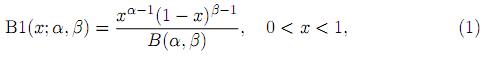
where α > 0 and β > 0, and

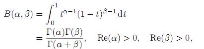
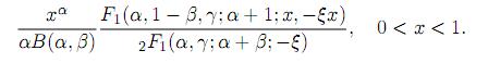
denotes the beta function. The beta distribution is very versatile and a variety of uncertainties can be usefully modeled by it. Many of the finite range distributions encountered in practice can easily be transformed into the standard beta distribution. Several univariate and matrix variate generalizations of this distribution are given in Gordy 1., Gupta and Nagar 2., Johnson, Kotz and Balakrishnan 3., McDonald and Xu 4., and Nagar and Zarrazola 5.. A natural univariate generalization of the beta distribution is the Gauss hypergeometric distribution defined by Armero and Bayarri 6.. The random variable X is said to have a Gauss hypergeometric distribution, denoted by X ∼ GH(α, β, γ, ξ), if its density function is given by

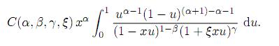
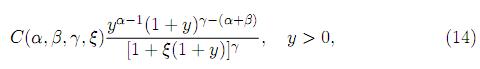
where α > 0, β > 0, −∞ < γ < ∞ and ξ > −1. The normalizing constant C(α, β, γ, ξ) is given by

where ₂F₁represents the Gauss hypergeometric function (Luke 7.). Note that the Gauss hypergeometric function ₂F₁ in (3) can be expanded in series form if −1 < ξ < 1. However, if ξ > 1, then we use suitably (7) to rewrite ₂F₁ to have absolute value of the argument less than one.

The above distribution was suggested by Armero and Bayarri 6. in connection with the prior distribution of the parameter ρ, 0 < ρ < 1, which represents the trafic intensity in a M/M/1 queueing system. A brief introduction of this distribution is given in the encyclopedic work of Johnson, Kotz and Balakrishnan 3, p. 253.. In the context of Bayesian analysis of unreported Poisson count data, while deriving the marginal posterior distribution of the reporting probablity p, Fader and Hardie 8. have shown that q = 1 − p has a Gauss hypergeometric distribution. The Gauss hypergeometric distribution has also been used by Dauxois 9. to introduce conjugate priors in the Bayesian inference for linear growth birth and death processes. Sarabia and Castillo 10. have pointed out that this distribution is conjugate prior for the binomial distribution.

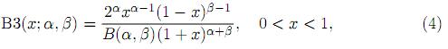
Gauss hypergeometric distribution reduces to a beta type 1 distribution when either γ or ξ equals to zero. Further, for γ = α +β and ξ = 1, the Gauss hypergeometric distribution simplifies to a beta type 3 distribution given by the density (Cardeño, Nagar and Sánchez 11., Sánchez and Nagar 12.),

where α > 0 and β > 0. For γ = α + β and ξ = −(1 − λ) it slides to a three parameter generalized beta distribution defined by the density

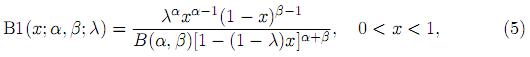
where α > 0 and β > 0. This distribution was defined and used by Libby and Novic 13. for utility function fitting. The beta distribution sometimes does not provide suficient flexibility for a prior for probability of success in a binomial distribution. Among various properties, the distribution defined by the density (5) can more flexibly account for heavy tails or skewness, and it reduces to the ordinary beta (type 1) distribution for certain parameter choices. The resulting posterior distribution in this case is a four-parameter type of beta. Chen and Novic 14. provided tables as evidence for its usefulness. Several properties and special cases of this distribution are given in Johnson, Kotz and Balakrishnan 3, p. 251.. For further results and properties, the reader is referred to Aryal and Nadarajah 15., Nadarajah 16., Nagar and Rada-Mora 17., Pham-Gia and Duong 18., and Sarabia and Castillo 10..

In this article, we derive distributions of the product and the ratio of two independent random variables when at least one of them is Gauss hypergeometric. We also study several properties of this distribution including Rényi and Shannon entropies.

 

2 Some Known Definitions and Results

In this section, we give definitions and results that are used in subsequent sections. Throughout this work we will use the Pochhammer coeficient (a)_n defined by (a)_n= a(a+1) · · · (a+n−1) = (a)_n−1(a+n−1) for n = 1, 2, . . . , and (a)₀ = 1. The integral representation of the Gauss hypergeometric function is given as

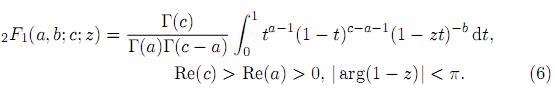
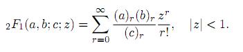
Note that, by expanding (1 − zt)_−b,|zt| < 1, in (6) and integrating t, the series expansion for ₂F₁can be obtained as

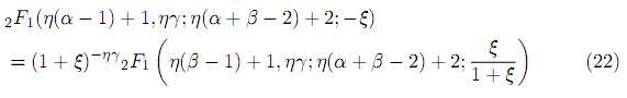
The Gauss hypergeometric function ₂F₁ (a, b; c; z) satisfies Euler's relation

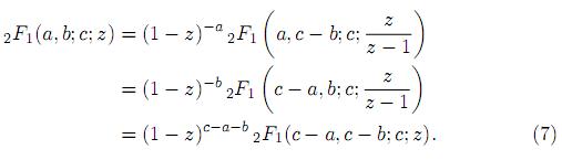
For properties and further results the reader is referred to Luke 7..

The Appell's first hypergeometric function F₁ is defined by

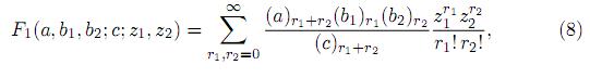
where |z₁|< 1 and |z₂|< 1. It is straightforward to show that

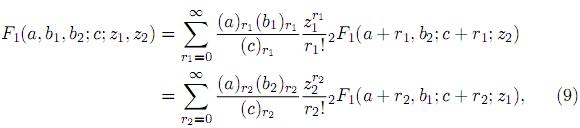
where ₂F₁ is the Gauss hypergeometric series. Using the results

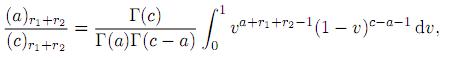
where Re(c) > Re(a) > 0,

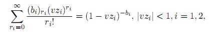
in (8), one obtains

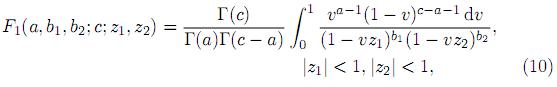
where Re(c) > Re(a) > 0. Note that for b₁ = 0, F₁ reduces to a ₂F₁ function. For properties and further results of these function the reader is referred to Srivastava and Karlsson 19..

Lemma 2.1. Let

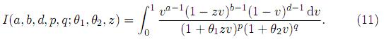
Then, for a > 0, d > 0 and 0 < z < 1, we have

Proof. Writing

and

in (11) and substituting v = 1 − w, we obtain

Now, using the definition of the Appell's first hypergeometric function, we get the desired result.

 

3 Properties

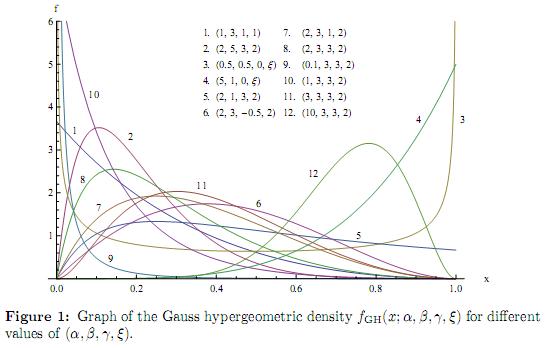
The graph of the Gauss hypergeometric density for different values of the parameters is shown in the Figure 1.

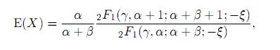
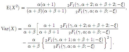
The k-th moment of the variable X having Gauss hypergeometric distribution, obtained in Armero and Bayarri 6., can be calculated as

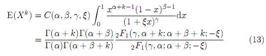
from which the expected value and the variance of this distribution are obtained as

Moreover, the cumulative distribution function (CDF) can be derived in terms of special functions as shown in the following theorem.

Theorem 3.1. Let X ∼ GH(α, β, γ, ξ). Then, the CDF of X is given by

Proof. The CDF of X is evaluated as

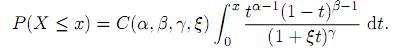
By making the substitution u = t/x, we can express the above integral as

Now, using the integral representation (10) of F₁, substituting for C(α, β, γ, ξ) from (3) and simplifying, we obtain the desired result.

The following theorem suggests a generalized beta type 2 distribution, from the Gauss hypergeometric distribution.

Theorem 3.2. Let X ∼ GH(α, β, γ, ξ). Then, the pdf of the random variable Y = X/(1 − X) is given by

where C(α, β, γ, ξ) is the normalizing constant given by (3).

Proof. Making the transformation Y = X/(1 − X), with the Jacobian J(x → y) = (1 + y)⁻² in (2), we get the desired result.

As expected, if in the density (14) we take γ = 0 or ξ = 0 with β > γ, then we obtain the beta type 2 density.

 

4 Entropies

In this section, exact forms of Rényi and Shannon entropies are obtained for the Gauss hypergeometric distribution defined in Section 1.

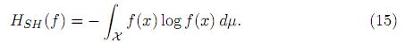
Let () be a probability space. Consider a pdf f associated with , dominated by σ−finite measure µ on . Denote by H_SH (f ) the well-known Shannon entropy introduced in Shannon 20. It is defined by

One of the main extensions of the Shannon entropy was defined by Rényi 21. This generalized entropy measure is given by

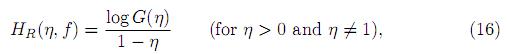
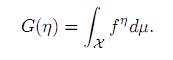
where

The additional parameter η is used to describe complex behavior in probability models and the associated process under study. Rényi entropy is monotonically decreasing in η, while Shannon entropy (15) is obtained from (16) for η ↑ 1. For details see Nadarajah and Zografos 22., Zografos 23., and Zografos and Nadarajah 24..

First, we give the following lemma useful in deriving these entropies.

Lemma 4.1. Let g(α, β, γ, ξ) = lim_η→1 h(η), where

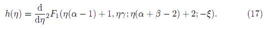
Then, for −1 < ξ < 1, we have

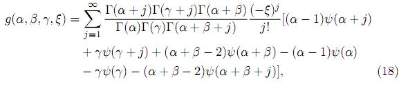
and for ξ ≥ 1,

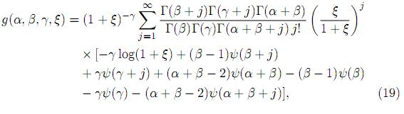
where ψ(z) = Γ´(z)/Γ(z) is the digamma function.

Proof. Using the series expansion of ₂F₁, for −1 < ξ < 1, we write

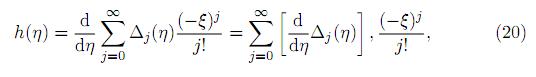
where

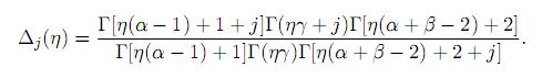
Now, differentiating the logarithm of Δ_j(η) w.r.t. η, we arrive at

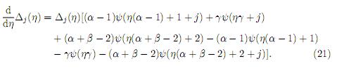
Finally, substituting (21) in (20) and taking η → 1, we obtain (18). To obtain (19), we use (7) to write

and proceed similarly.

Theorem 4.1. For the Gauss hypergeometric distribution defined by the pdf (2), the Rényi and the Shannon entropies are given by

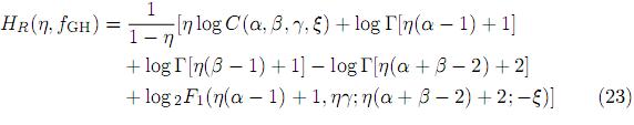
and

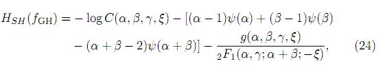
respectively, where for −1 < ξ < 1, g(α, β, γ, ξ) is given by (18), and for ξ ≥ 1 g(α, β, γ, ξ) is given by (19).

Proof. For η > 0 and η ≠ 1, using the density of X given by (2), we have

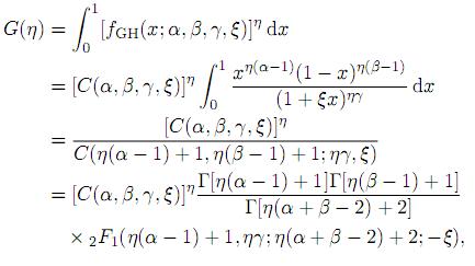
where the last line has been obtained by using (3). Now, taking logarithm of G(η) and using (16) we get (23). The Shannon entropy is obtained from (23) by taking η ↑ 1 and using L'Hopital's rule.

 

5 Distribution of The Product

In this section, we obtain distributional results for the product of two independent random variables involving Gauss hypergeometric distribution.

Theorem 5.1. Let X₁ and X₂ be independent, Xi∼ GH(α_i, β_i, γ_i, ξ_i), i = 1, 2. Then, the pdf of Z = X₁X₂ is given by

where

Proof. Using the independence, the joint pdf of X₁ and X₂ is given by

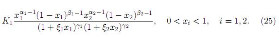
Transforming Z = X₁X₂, X₂ = X₂ with the Jacobian J(x₁, x₂ → z, x₂) = 1/x₂, we obtain the joint pdf of Z and X₂ as

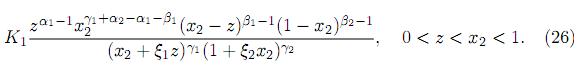
To find the marginal pdf of Z, we integrate (26) with respect to x₂ to get

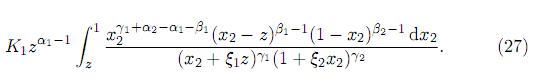
In (27) change of variable w = (1 − x₂)/(1 − z) yields

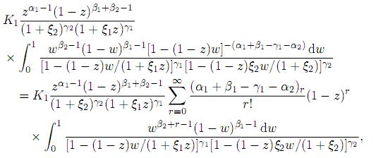
where the last step has been obtained by expanding 1−(1−z)w.−^{(α₁+β₁−γ₁−α₂)} in power series. Finally, applying (10), we obtain the desired result.

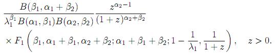
Corollary 5.1.1. Let X₁ ∼ GH(α₁, β₁, γ₁, ξ₁) and X₂ ∼ B1(α₂, β₂) be independent. Then, the pdf of Z = X₁ X₂ is

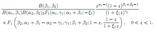
Proof. Substituting γ₂ = 0 in Theorem 5.1 and using (9) we get the desired result.

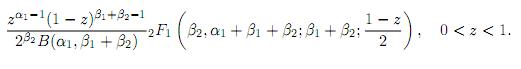
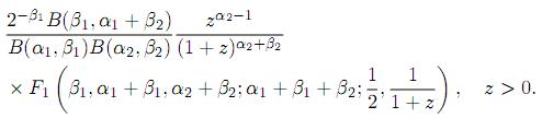
Corollary 5.1.2. Let the random variables X₁ and X₂ be independent, X₁ ∼ B1(α₁, β₁) and X₂∼ B3(α₂, β₂). If α₂= α₁+ β₁, then the pdf of Z = X₁X₂ is given by

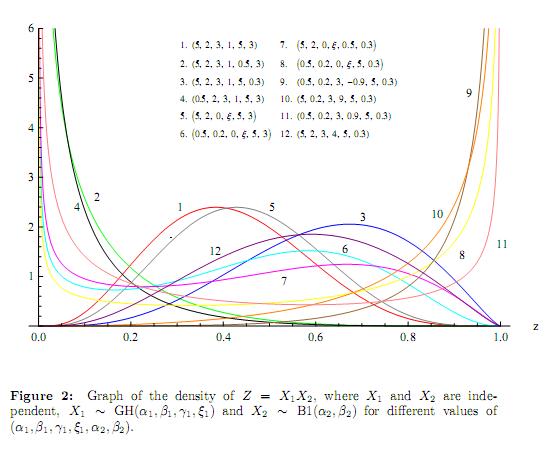
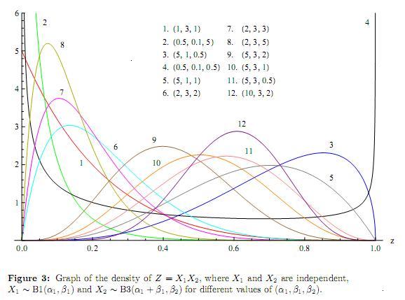
The graphs of the pdf of Z = X₁X₂, where X₁ and X₂ are independent, X₁ ∼ GH(α₁ , β₁, γ₁, ξ₁) and X₂ ∼ B1(α₂, β₂) for different values of (α₁, β₁, γ₁, ξ₁, α₂, β₂) for different values of the parameters is shown in the Figure 2. Further, Figure 3 depicts graphs of the density of Z = X₁X₂, where X₁ and X₂ are independent, X₁ ∼ B1(α₁, β₁) and X₂ ∼ B3(α₁ + β₁, β₂) for different values of (α₁, β₁, β₂).

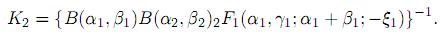
Theorem 5.2. Let the random variables X₁ and X₂ be independent, X₁ ∼ GH(α₁, β₁, γ₁, ξ₁) and X₂ ∼ B2(α₂, β₂). Then, the pdf of Z = X₁X₂ is given by

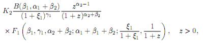
where

Proof. Since X₁ and X₂ are independent, their joint pdf is given by

Now consider the transformation Z = X₁X₂, W = 1 − X₁ whose Jacobian is J (x₁, x₂ → w, z) = 1/(1 − w). Thus, we obtain the joint pdf of W and Z as

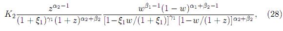
where z > 0 and 0 < w < 1. Finally, integrating w using (10) and substituting for K₂ in (28), we obtain the desired result.

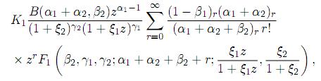
Corollary 5.2.1. Let the random variables X₁ and X₂ be independent, X₁ ∼ B1(α1, β1; λ1) and X₂∼ B2(α₂, β₂). Then, the pdf of Z = X₁X₂ is given by

 

Corollary 5.2.2. Let the random variables X₁ and X₂ be independent, X₁ ∼ B1(α₁, β₁) and X2 ∼ B2(α₂, β₂). Then, the pdf of Z = X₁X₂ is given by

Corollary 5.2.3. Let the random variables X₁ and X₂ be independent, X₁ ∼ B3(α₁, β₁) and X₂ ∼ B2(α₂, β₂). Then, the pdf of Z = X₁X₂ is given by

 

6 Distribution of The Quotient

In this section we obtain distributional results for the quotient of two independent random variables involving Gauss hypergeometric distribution.

In the following theorem, we consider the case where both the random variables are distributed as Gauss hypergeometric.

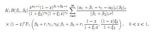
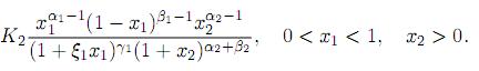
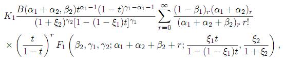
Theorem 6.1. Let the random variables X₁ and X₂ be independent, X_i∼ GH(α_i, β_i, γ_i, ξ_i), i = 1, 2. Then, the pdf of Z = X₁/X₂ is given by

for 0 < z ≤ 1, and

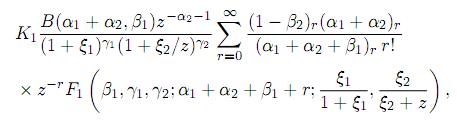
for z > 1.

Proof. The joint pdf of X₁ and X₂ is given by (25). Now, transforming Z = X₁/X₂ , V = X₂ with the Jacobian J(x₁, x₂ → z, v) = v, we obtain the joint pdf of Z and V as

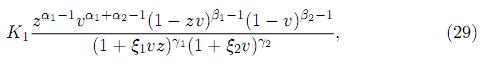
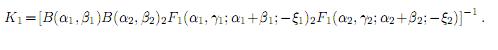
where 0 < v < 1 for 0 < z ≤ 1, and 0 < v < 1/z for z > 1. For 0 < z ≤ 1, the marginal pdf of Z is obtained by integrating (29) over 0 < v < 1. Thus, the pdf of Z, for 0 < z ≤ 1, is obtained as

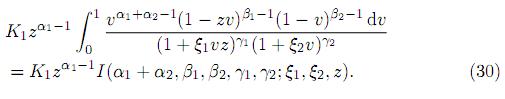
Now, using Lemma 2.1 and substituting K₁ in the density (30) we get the desired result. For z > 1, the density of Z is given by

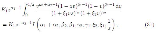
where the last line has been obtained by substituting w = vz. Finally, using Lemma 2.1 and substituting for K₁, we obtain the pdf of Z for z > 1.

Theorem 6.2. Let the random variables X₁ and X₂ be independent, X_i ∼ GH(α_i, β_i, γ_i, ξ_i), i = 1, 2. Then, the pdf of T = X₁ /(X₁ + X₂) is given by

for 0 < t ≤ 1/2, and

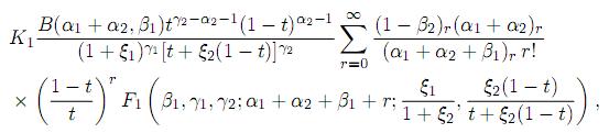
for 1/2 < t < 1.

Proof. Making the transformation T = Z/(1 + Z) with the Jacobian J(z → t) = (1 − t)⁻² in Theorem 6.1 we get the desired result

 

Acknowledgment

This research work was supported by the Comité para el Desarrollo de la Investigación(CODI), Universidad de Antioquia research grant no. IN560CE.

 

References

1. Michael B. Gordy. Computationally convenient distributional assumptions for common-value auctions. Computational Economics, ISSN: 0927–7099, EISSN: 1572–9974, 12(1), 61–78 (1998). 30        [ Links ]

2. A. K. Gupta and D. K. Nagar. Matrix variate distributions. Chapman & Hall/CRC Monographs and Surveys in Pure and Applied Mathematics, 104, ISBN: 1-58488-046-5, Chapman & Hall/CRC, Boca Raton, FL, 2000. 30        [ Links ]

3. N. L. Johnson, S. Kotz and N. Balakrishnan. Continuous univariate distributions. Vol. 2. Second edition, Wiley Series in Probability and Mathematical Statistics: Applied Probability and Statistics. A WileyInterscience Publication, ISBN: 978-0-471-58494-0, John Wiley & Sons, Inc., New York, 1995. 30, 31, 32        [ Links ]

4. J. B. McDonald and Y. J. Xu. A generalization of the beta distribution with applications. Journal of Econometrics, ISSN: 0304-4076, 66(1&2), 133–152 (1995). 30        [ Links ]

5. D. K. Nagar and E. Zarrazola. Distributions of the product and the quotient of independent Kummer-beta variables. Scientiae Mathematicae Japonicae, ISSN: 1346–0862, EISSN: 1346–0447, 61(1), 109–117 (2005). 30        [ Links ]

6. C. Armero and M. Bayarri. Prior assessments for predictions in queues. The Statistician, ISSN: 1467–9884, 43(1), 139–153 (1994). 30, 31, 35        [ Links ]

7. Y. L. Luke. The special functions and their approximations, Vol. I. Mathematics in Science and Engineering, Vol. 53, ISBN: 0-124-59901-X, Academic Press, New York-London, 1969. 31, 33        [ Links ]

8. Peter S. Fader and Bruce G. S. Hardie. A note on modelling underreported Poisson counts. Journal of Applied Statistics, PISSN: ISSN: 0266-4763, OISSN: 1360-0532, 27(8), 953–964 (2000). 31         [ Links ]

9. J.-Y. Dauxois. Bayesian inference for linear growth birth and death processes. Journal of Statistical Planning and Inference, ISSN: 0378-3758, 121(1), 1–19 (2004). 31        [ Links ]

10. José María Sarabia and Enrique Castillo. Bivariate distributions based on the generalized three-parameter beta distribution. Advances in distribution theory, order statistics, and inference, ISBN: 978-0-8176-4361-4, 85–110, Stat. Ind. Technol., Birkhäuser Boston, Boston, MA, 2006. 31, 32        [ Links ]

11. Liliam Cardeño, Daya K. Nagar and Luz Estela Sánchez. Beta type 3 distribution and its multivariate generalization. Tamsui Oxford Journal of Mathematical Sciences, ISSN: 1561-8307, 21(2), 225–241 (2005). 31        [ Links ]

12. Luz E. Sánchez and Daya K. Nagar. Distributions of the product and quotient of independent beta type 3 variables. Far East Journal of Theoretical Statistics, ISSN: 0972-0863, 17(2), 239–251 (2005). 31         [ Links ]

13. D. L. Libby and M. R. Novic. Multivariate generalized beta distributions with applications to utility assessment. Journal of Educational Statistics, ISSN: 0362-9791, 7(4), 271–294 (1982). 32        [ Links ]

14. J. J. Chen and M. R. Novick. Bayesian analysis for binomial models with generalized beta prior distributions.Journal of Educational Statistics, ISSN: 0362-9791, 9, 163–175 (1984). 32        [ Links ]

15. Gokarna Aryal and Saralees Nadarajah. Information matrix for beta distributions. Serdica Mathematical Journal, ISSN: 1310-6600, 30(4), 513–526 (2004). 32        [ Links ]

16. Saralees Nadarajah. Sums, products and ratios of generalized beta variables. Statistical Papers, PISSN: 0932-5026, EISSN: 1613-9798, 47, (1), 69–90 (2006). 32        [ Links ]

17. Daya K. Nagar and Erika Alejandra Rada-Mora. Properties of multivariate beta distributions. Far East Journal of Theoretical Statistics, ISSN: 0972–0863, 24(1), 73–94 (2008). 32        [ Links ]

18. T. Pham-Gia and Q. P. Duong. The generalized beta and F -distributions in statistical modelling. Mathematics and Computer Modelling, ISSN: 0895-7177, 12(12), 1613–1625 (1989). 32        [ Links ]

19. H. M. Srivastava and P. W. Karlsson. Multiple Gaussian hypergeometric series, ISBN: 0-470-20100-2, Halsted Press John Wiley & Sons., New York, 1985. 33        [ Links ]

20. C. E. Shannon. A mathematical theory of communication. Bell System Technical Journal, ISSN : 0005-8580, 27, 379–423, 623–656 (1948). 37        [ Links ]

21. A. Rényi. On measures of entropy and information, Proceedings of the Fourth Berkeley Symposium on Mathematical Statistics and Probability, Volume 1: Contributions to the Theory of Statistics, ISSN: 00970433, University of California Press, Berkeley, California, pp. 547–561 (1961). 37        [ Links ]

22. S. Nadarajah and K. Zografos. Expressions for Rényi and Shannon entropies for bivariate distributions. Information Sciences, ISSN: 00200255, 170(2-4), 173–189 (2005). 37        [ Links ]

23. K. Zografos. On maximum entropy characterization of Pearson's type II and VII multivariate distributions. Journal of Multivariate Analysis, ISSN: 0047-259X, 71(1), 67–75 (1999). 37        [ Links ]

24. K. Zografos and S. Nadarajah. Expressions for Rényi and Shannon entropies for multivariate distributions. Statistics & Probability Letters, ISSN: 0167-7152, 71(1), 71–84 (2005). 37        [ Links ]