Salvador Ruz Rojas¹, Carlos-Humberto Amaya², and Alberto Mendoza³

¹Universidad Industrial de Santander, UIS -Grupo de Informática para Hidrocarburos-, Bucaramanga, Santander, Colombia. e-mail: salvador.ruz@gmail.com

^2,3Ecopetrol S.A. - Instituto Colombiano del Petróleo, A. A. 4185, Bucaramanga, Santander, Colombia

(Received Jun. 13, 2005; Accepted Sept. 8, 2006)

ABSTRACT. The assessment of the success of a stimulation job often has a lot of uncertainties caused by the different viewpoints assumed by engineers.

This paper presents a methodology to evaluate the success of workovers jobs, using common production data and well known equations.

For wells in pseudo-steady state flow, assuming that the oil rate can be extrapolated using decline curve analysis, the effectiveness of the stimulation job is quantified in terms of additional oil reserves, changes in productivity index, removed skin and profits.

A Matlab^TM software application was built to calculate the declining parameters and two examples in the Brisas field (an oilfield located at the Southwest of Colombia) are used to illustrate the methodology.

Keywords: well stimulation, production decline curve, well performance, job evaluation, productivity index, well pressure.

RESUMEN. La evaluación del éxito de un trabajo de estimulación presenta muchas incertidumbres debido a los diferentes enfoques asumidos por los ingenieros.

En este artículo se expone una metodología para evaluar el éxito de los trabajos de reacondicionamiento de pozo, utilizando datos de producción de uso habitual y ecuaciones de amplio uso en la industria del petróleo.

Asumiendo que el pozo se encuentra fluyendo a estado seudo-estable y que el caudal de aceite puede ser extrapolado utilizando el análisis de curvas de declinación, la efectividad de los trabajos de estimulación es cuantificada en términos de reservas adicionales de aceite, cambios en el índice de productividad, factor de daño removido y beneficios económicos.

Un software de aplicación fue construido en Matlab^TM para calcular los parámetros de declinación, y fueron utilizados dos ejemplos de aplicación en el campo Brisas (un campo ubicado al sur-occidente colombiano) para ilustrar la metodología.

Palabras clave: estimulación de pozos, curva de declinación de producción, desempeño del pozo, evaluación de trabajos, índice de productividad, presión de pozo.

INTRODUCTION

Although stimulation jobs evaluation is quite routine, it is normal to find uncertainties in the results caused by the different perspectives assumed by the engineers.

The objective of an oil well stimulation treatment and some type of workovers is mainly one: to improve the connection between the well and the desired reservoir fluids (Allen & Roberts, 1997). However, a treatment job can affect the well performance in different ways such as changing the oil rate, reducing the declining rate, increasing the reserves, among others. Therefore, a partial approach may cause uncertainties and subjectivities in the evaluation. For example, if the engineer calculates only the changes in the oil rate, the analysis may be affected by the artificial lift system performance.

This paper illustrates how to use simple well known equations and usual production data to calculate the additional oil barrels, the profits, and the delayed production, due to the stimulation. The proposed methodology assumes that the oil rate can be extrapolated using the Arps´ decline theory (Arps, 1949, 1956). Then, considering that the well is in pseudo-state flow, two equations are stated to calculate the removed skin.

ADDITIONAL OIL BARRELS

It is a common practice to use the change in the oil rate, rate before and after the treatment, as a first glance evaluation of the stimulation effectiveness. In every evaluation report it is quite normal to find information about production tests before and after the job, but this kind of analysis is not complete because depicts the well flowing capacity in a snapshot manner.

To see the entire effect of the stimulation it is necessary to include an important factor: the stimulation job performance as a function of time.

A well stimulation can cause an increase in the oil rate, but that does not guarantee that the effect lasts. Some workover jobs seem to be excellent because they provide excellent results at the beginning, but it can happen that few weeks later, negative effects, such as water incoming or a drastic reduction in the oil rate may appear.

Another kind of treatments e.g., scale inhibition, does not reduce damage but avoid future flowing blockage. So they have a positive effect in the well performance and must be valued as good ones, because they enhance oil reserves, no matter there is no oil rate increase. In order to quantify the effect of a treatment in a long time perspective, not only the rate changes but also additional oil barrels should be computed.

Decline Curve Analysis (DCA)

If a clear production trend can be established and if this tendency can be extrapolated using the Arp’s decline equations (Arps, 1949, 1956), the additional barrels due to the entire workover job can be measured.

There are several commercial software packages to forecast oil rates based on DCA but in this paper, the forecasted oil rates were determined using an in-house software developed in Matlab^TM. The application use non-linear regression and the minimum square algorithm to determine the hyperbolic and the exponential decline parameters, respectively (Ruz & Calderón, 2005).

Additional oil barrels are the difference between the actual cumulative oil barrels and the barrels obtained if the stimulation job had not been performed.

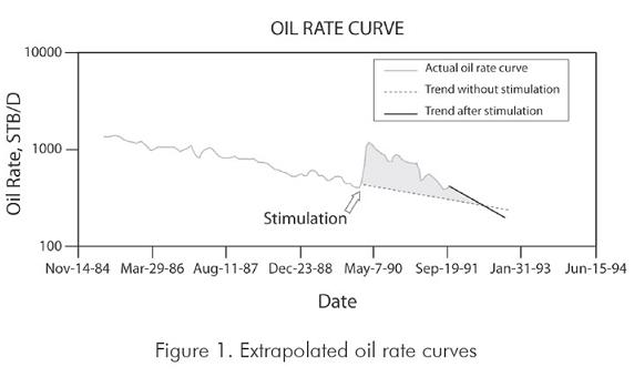
Figure 1 is a graphical explanation of the explanation of the decline curve analysis step. Note that the dashed line in Figure 1 represents the oil rate obtained if the stimulation job is not performed. The solid black line in Figure 1 represents a second extrapolation of oil rates when there is not enough data or when the well have been affected by a further event. The grey area is the additional cumulative oil due to the stimulation. It can be observed that after the black line intercepts the dashed line, the treatment becomes unfavorable. The management team should achieve another workover before this situation takes place, if it is economically feasible.

In the cumulative oil curve, the additional cumulative oil is not an area, but the difference between the actual and the expected behavior without the stimulation (see delta Noil in Figure 2). This cumulative curve helps verifying if the oil rates were extrapolated correctly, which means reducing subjectivity and promoting precision.

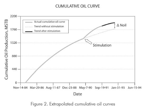
Note: Although in the International System of Units the prefix k (kilo) stands for thousands, it will be used MSTB to represents thousands of oil barrels, because that is the way it is named in the oil industry.

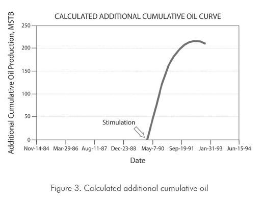
In relation to Figure 2, the Additional Cumulative Oil Curve (ACOC) can be seen as delta Noil as a function of time (Figure 3). Note that the highest value in Figure 3 is the point where the black line intercepts the dashed line in Figure 1.

Deferred production

To execute a workover, the oil well production has to be stopped. Consequently, the delayed production is a kind of cost that has to be "charged" to the workover (or the stimulation) and its value should be deducted from the additional cumulative oil.

The deferred production can be calculated using the last reported oil rate just before the stimulation times the workover duration (Equation 1).

DP_o = q_{o_jbt} * WK_time (1)

Types of curves

Based on the shape of the production oil curves, there are five types of workovers (Figures 4 and 5):

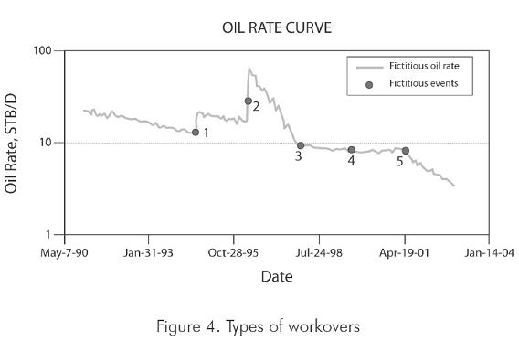
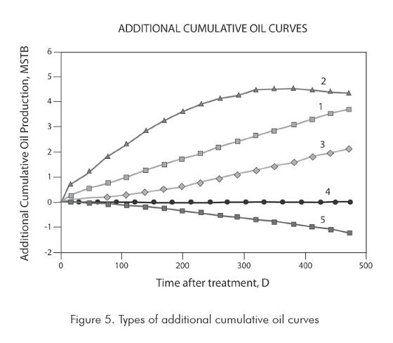
1. The oil rate increases and the declining trend stays equal or favorable.

2. The oil rate increases but the declining trend gets worse.

3. The oil rate does not increase and the declining trend changes favorably.

4. The workover does not cause any effect.

5. The event causes production impairment just after the treatment.

Figure 5 illustrates the additional cumulative oil curves that would result from the several cases in Figure 4.

PROFITS

The stimulation job effectiveness is not strictly based on additional oil barrels. Profits are affected by factors such as treatment costs e.g., acid treatments are usually cheaper than hydraulic fracturing. Therefore, the net profit should be computed and included in the workover appraisal.

Elapsed time point of view

From the gray area in Figure 1, the additional oil barrels calculation seems to be an integral calculus problem. Fortunately, production data has to be reported in an elapsed time way, so the problem is purely discrete (not continuous). This means that the additional oil barrels and the profits calculations can be estimated as the summation of monthly fractions.

For example, if an oil well has the production reported in the Table 1, to estimate the monthly profits it is only necessary to multiply the monthly additional oil barrels by the profits per barrel (profit per sold oil barrel).

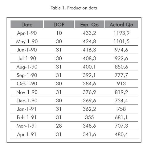
In Table 1 DOP, Exp. Qo and Actual Qo means days on production, the expected oil rate if the stimulation is not performed (STB/D) and the actual oil rate after the stimulation (STB/D), respectively.

In Table 2, the column MAOB contains the monthly additional oil barrels (Equation 2).

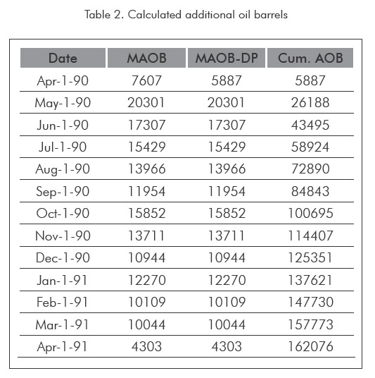
MAOB = (q_{o_act} - q_{o_exp}) * DOP (2)

The column MAOB-DP contains the monthly additional oil barrels minus the deferred production. Assuming that the last oil rate just before the treatment was 430 STB/D, and that the stimulation lasts four days, the deferred production is 1720 oil barrels (it means that the deferred production is totally recovered in the first month after the job).

The column Cum. AOB contains the cumulative additional oil barrels (note the deferred production was already deducted).

If the profit in dollars per sold barrel (column PPSB in Table 3) is known, it is straightforward to compute the monthly profit using Equation 3.

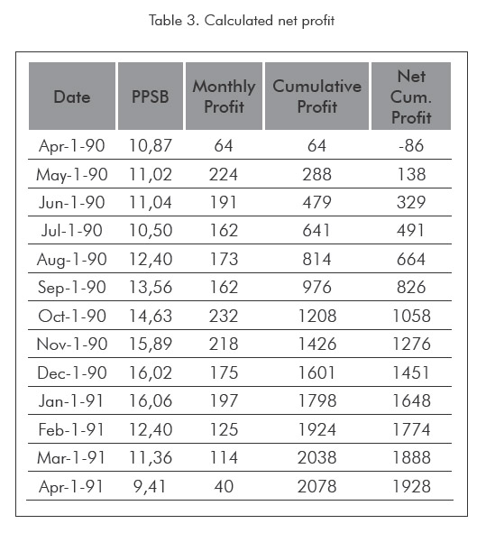
Monthly Profit = (MAOB - DP_o) * PPSB (3)

The third column Monthly Profit in Table 3 is the monthly revenue in thousands of dollars and the fourth column Cum. Profit contains the cumulative profits. If the treatment cost US$ 150 000, the investment is recovered in about one and a half month.

The column Net Cum. Profit contains the cumulative net profit in thousands of dollars that is the cumulative profit less the treatment cost.

This kind of economical analysis is not complete. To improve it, the present value profit (PVP) and the profit-to-investment ratio (P/I) must be included; therefore it is advisable to see the Patterson’s technique (Patterson, 1973) to exhibit the profits in proper economical terms.

REMOVED SKIN

The difference between the skin factor before and after the treatment can be considered as the removed skin. Pressure tests before and after the workover is the best mechanism to calculate the removed skin. Unfortunately, it is not a common practice to run tests regularly.

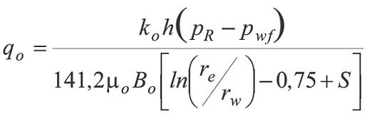
To overcome this difficulty, it can be derived, from the equation for pseudo-steady state flow (Equation 4), a relationship between the skin before and after the treatment (Golan & Whitson, 1991).

(4)

According to Equation 4, the expected oil rate without performing a treatment can be expressed as:

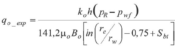(5)

And the actual oil rate can be expressed as:

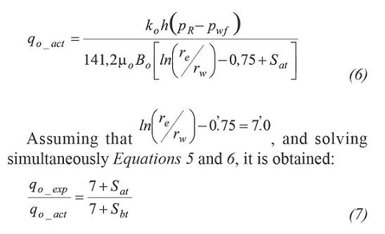(6)

Assuming that , and solving simultaneously Equations 5 and 6, it is obtained:

(7)

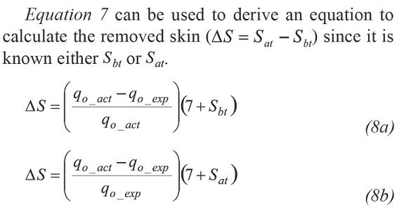
Equation 7 can be used to derive an equation to calculate the removed skin (AS = S_at - S_bt) since it is known either S_bt or S_at.

(8a)

In Equations 8a and 8b, the rate is the oil rate (not the total rate) because including the water rate can deceive the analysis.

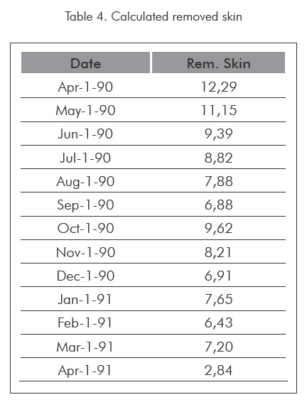
When the treatment removes the total skin, Equation 8b can be used to calculate because in that case is equal to zero.

As an example, assuming that from a well test S_at= 0, Equation 8b is used to compute the removed skin for the data listed in Table 1 (see column Rem. Skin in Table 4).

PRODUCTIVITY INDEX ANALYSIS (PIA)

Until this point, the evaluation has been based on production data. This approach has a drawback because oil extraction depends on the Artificial Lift System (ALS) design and performance.

To see properly the effect of the treatment in the well flowing capacity, it is necessary to check the productivity index (Equation 9). The treatment is effective if after the job, the productivity index increase.

(9)

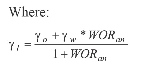
As stated before, if the analysis uses the total (oil and water) rate, the water can mislead the evaluation. So, it is better to check oil productivity index and water productivity index separately. In this way, it is possible to identify water breakthrough.

Bottomhole flowing pressure estimation

The productivity index valuation requires the drawdown and consequently the flowing pressure. If the well does not have a downhole pressure recording device, the flowing pressure can be calculated from the fluid level, using basic hydrostatic relationships.

Assuming that the fluid is static in the tubing-casing annulus, the flowing pressure can be calculated from both the casing pressure and the pump intake pressure (Figure 6).

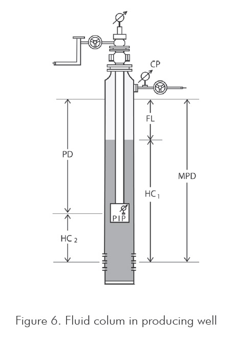
From the casing pressure, and using the Gilbert Equation (Golan & Whitson, 1991), the relationship to estimate the flowing pressure is:

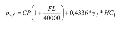(10)

Where:

(10a)

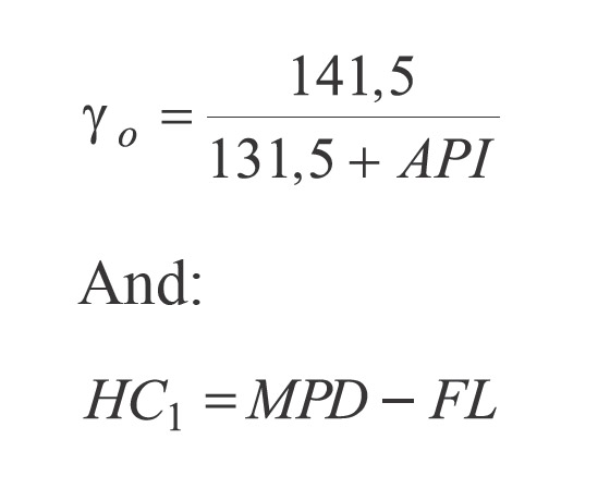(10b)

From the pump intake pressure the relationship to estimate the flowing pressure is:

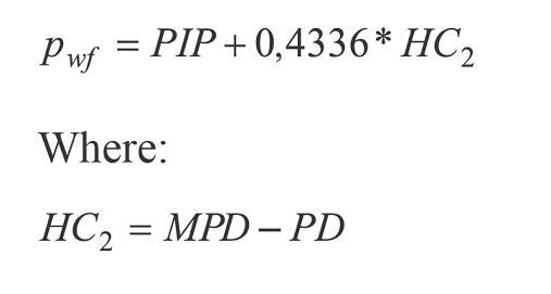(11)

Same Drawdown Criteria (SDC).

As the fluid level depends on both the ALS and the well performance, the pressure drawdown may change after the treatment.

To make clear the effect of the treatment in the well performance (avoiding ALS effects), the same drawdown criteria must be applied. That is, from the productivity index after the treatment and using the pressure drawdown before the stimulation, the stimulated same drawdown oil rate is calculated (Equation 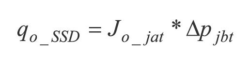12).

(12)

It is advisable to use the SDC only to quantify the Instantaneous Workover Efficiency (IWE), because it is difficult to predict appropriately the well production merely extrapolating the productivity index and the pressure drawdown (elevated drawdown can cause, for example, water coning, fines migration, etc). Consequently, it is not recommended to calculate the additional oil barrels due to the workover using the SDC.

In IWE the word instantaneous means the workover effect that results from comparing oil rates just before and just after the treatment.

EXAMPLES IN THE BRISAS FIELD

The Brisas field (Paez, Gsmez, Saavedra, Mendoza, & Pérez, 2003) was discovered in 1973 by Tenneco Company and nowadays is operated by Ecopetrol S.A. This field is located at the Southwest of Colombia in the upper Magdalena basin and produces oil crude from the Monserrate formation. The average true vertical depth of the wells is 4300 feet and the production mechanism is a combination of solution gas drive and partial water drive.

The API gravity is 23 and the bubble pressure is approximately 800 psi. The reservoir pressure was 2000 psi in 1973 and 900 psi in 2003.

The formation damage is caused mainly by calcium carbonate scale. This damage mechanism has been deducted by the calculated saturation index for calcite and confirmed by the effectiveness of HCl treatments. calcium carbonate scale also has been found in the production string.

Treatment analysis in Brisas-9

Following the additional oil barrels perspective, three acid-organic stimulations (Figure 7) were evaluated in the well Brisas-9 oil.

The gas-oil ratio (GOR) in Brisas-9 has ranged from 17 to 303 scf/stb.

According to the drive mechanism in the Brisas field and checking the oil rate data, it is clear that an exponential decline curve can be used in the evaluation. Figure 8 shows the areas calculated using DCA.

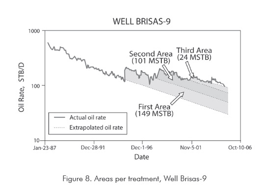
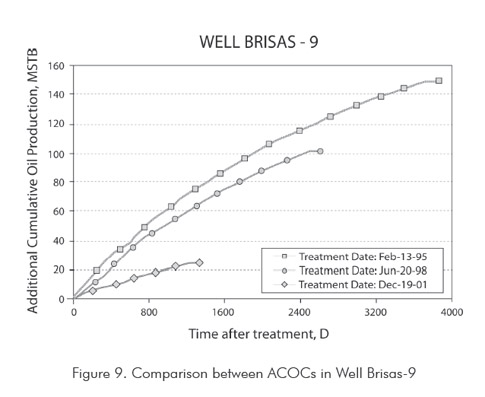
Figure 9 contains the additional cumulative oil curves for the analyzed stimulation jobs. To make the comparison between stimulations, the ACOC’s were plotted using as the abscissa the days after the treatment.

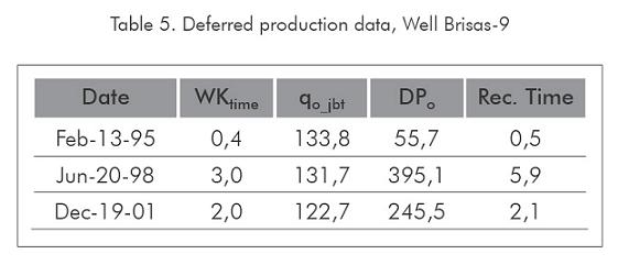
In Table 5 appears the deferred production for each workover. The column Rec. Time contains the time (in days) needed to recover the deferred production.

From Figure 9, it is comprehensible that similar treatments applied in the same well can gives different results. In this case, the acid-organic treatment was less effective in December 2001 than in February 1995, because the flow potential of the well was changing according to the reservoir depletion.

To calculate the removed skin it is necessary to have at least one skin value near (just before or just after) the treatment date. In Brisas-9 there was only one pressure test (July 1991 and the skin calculated was 1,1). Because of this lack of information, the skin at January 1995 is estimated using the flow efficiency equation (Golan & Whitson, 1991).

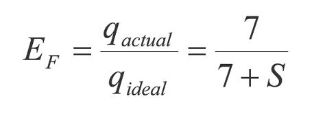(13)

Calculating the ideal rate at July 1991 (from Equation 13), the skin factor at January 1995 can be approximated to 4,83 (Calculations of removed skin and approximated skin were made in oil-rate basis, which means, it was assumed no multiphase flow effects).

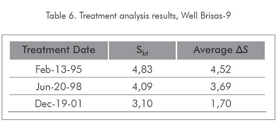
Figure 10 illustrates the removed skin calculated using Equation 8a. According to this figure, the first treatment analyzed in Brisas-9 well, removed an average skin damage of 4,52. Therefore, the skin factor after this treatment should be around 0,31. Using again Equation 13, the skin at June 1998 was approximately 4,09. The same steps are repeated to find the average removed skins for each treatment. A summary of this results appears in Table 6.

Treatment analysis in Brisas-8

In the Brisas field the fluid level information has been recorded since September 1997. Therefore, two stimulations, performed after that date, were evaluated to illustrate the productivity index analysis.

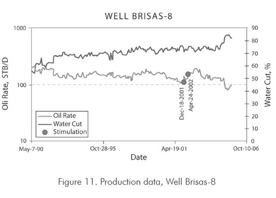
The first one is an organic-acid treatment (10 bbl xylene plus 10 bbl diesel plus 29 bbl 7,5% HCl) performed in November 2001. The second one is an acid treatment (8 bbl of 7.5% HCl) performed in April 2002 (Figure 11).

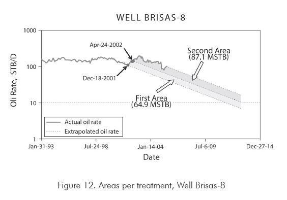
The evaluation of this well starts with the additional cumulative oil curves. (Figures 12 and 13).

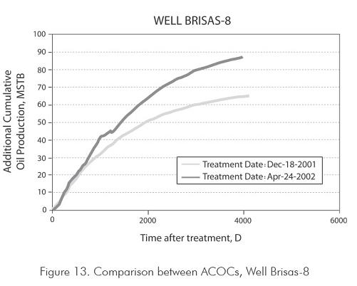
Until this step of the evaluation, the second stimulation (Apr. 24, 2002) was better than the first one. However, the PIA will help to understand the actual stimulation effects.

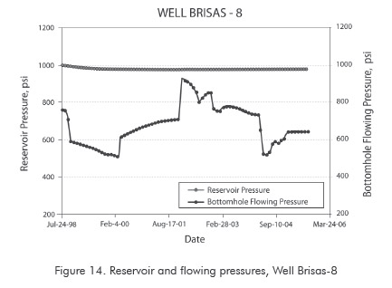
The flowing pressure was calculated from the fluid levels, and the reservoir pressure was obtained from different pressure test (Figure 14).

The productivity index was estimated from oil and water rates separately (Figure 15). From Figure 15 it can be concluded that the first stimulation (Dec. 18, 2001) caused a production increase but the second stimulation (Apr. 24, 2002) had no effect in the productivity index, thus its effect in the oil rate curve must be the result of an ALS change.

In addition to the productivity index, analysis of the treatment effluents can be used to determine if the stimulation removed or not any organic or inorganic flow obstruction. However, that topic is out of the scope of this paper.

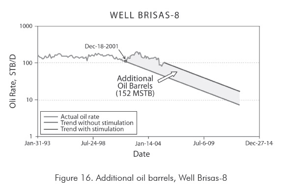
Finally, to complete the evaluation in the Brisas-8, the entire additional oil increase will be assigned to the first stimulation job (Figure 16).

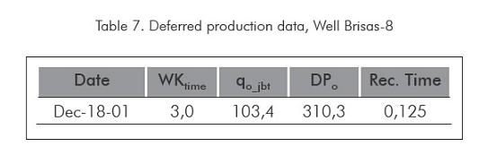
The deferred production is listed in Table 7.

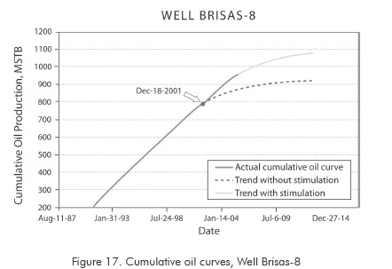
An extrapolated cumulative oil curve is showed in Figure 17.

The additional cumulative oil curve is plotted in Figure 18.

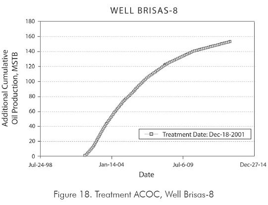
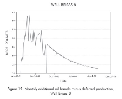
The profits were calculated using the monthly additional oil barrels (Equation 2), the deferred production (Equation 1) and the profits per sold barrel.

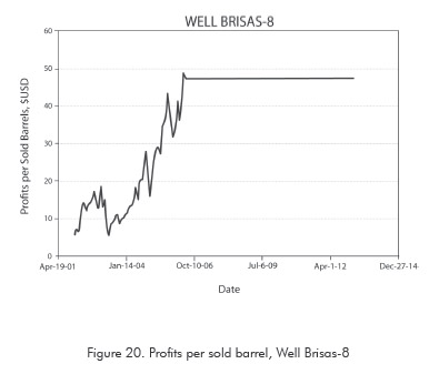
Figure 19 illustrates the calculated monthly additional oil barrels minus deferred production. The profits per sold barrel (Figure 20) were calculated taking into account oil prices and cost operations (note that the information contained in Figure 20 is fictitious and does not represent exactly the profits per sold barrel for the Brisas field).

Monthly profits, calculated using Equation 3, are plotted in Figure 21.

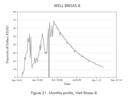
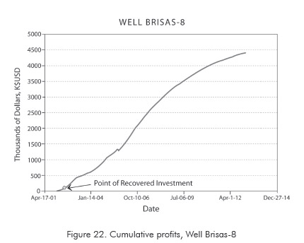
The date to recover the investment can be estimated from the cumulative profits curve (Figure 22). Assuming that the treatment cost 100 K$USD, the investment is recovered in 6,5 months.

DISCUSSION

A workover evaluation based in the DCA and the pseudo-steady state assumption is appropriate because it can be applied using common production data. In general, a more sophisticated solution, such as that generated using simulation, may not be cost-effective. The Arp´s decline curve can be established using a group of rate data collected for an elapsed time when no major changes in operating procedure are made and no stimulation treatments are applied (Arps, 1956). This condition is found in many wells; however, every case should be analyzed separately to verify if the well accomplishes the constraints. Because of the oil rate can be affected by the performance of the artificial lift system, the productivity index analysis should be included in the treatment evaluation. It is suggested to make productivity index calculations for water and oil separately, because in this way it is easier to detect water breakthrough. However, this implies that the relative permeability effect is neglected. To improve the proposed methodology it is recommended to include aspects such as workover operation, treatment formulation, and net present value of the revenues.

CONCLUSIONS

• If a clear production trend can be established and described by the Arp’s decline theory, the effectiveness of a stimulation treatment can be calculated using well known equations and common production data.

• Assuming the pseudo-steady state flow and calculating hydrostatic pressures in the well annulus, factors such as the artificial lift system performance and the removed skin damage, can be included in the analysis to avoid misleading results.

ACKNOWLEDGEMENTS

Many ideas in this paper are the result of discussions with colleagues at Ecopetrol S.A. The authors of this paper wish to express their gratitude to the ICP´s customers from whom we have received many valuable ideas, especially to Hugo-Iván Muñoz Añazco, Javier-Darío Páez, Jorge Hernández Mora and Iván Fedullo Rumbo.

REFERENCES

Allen, T. O., & Roberts A. P. (1997). Production operations (Vol. 2., 4th Ed.). Oil & Gas Consultants Internacional Inc. Tulsa Oklahoma, USA.        [ Links ]

Arps, J. J. (1949). Analysis of decline curves. Trans. AIME, 186: 9.         [ Links ]

Arps, J. J. (1956). Estimation of primary oil reserves. Trans. AIME, 207: 182-191.         [ Links ]

Golan, M., & Whitson, C. H. (1991). Well Performance. (2nd. ed.) Prentice Hall, Englewoods Cliffs, NJ.         [ Links ]

Páez, J. D., Gsmez, M.P., Saavedra, N. F., Mendoza, A., & Pérez, E. R. (2003). Formation damage study in the Brisas Field. Internal Report, Instituto Colombiano del Petrsleo -ICP, Ecopetrol S.A.         [ Links ]

Patterson, W. E., & Shell Oil Co. (1973). An economic evaluation technique for workovers with declining production. Fall Meeting, SPE, Las Vegas, USA, SPE 4618.         [ Links ]

Ruz, S., & Calderón, Z. (2005). Reserves estimation and hyperbolic decline parameters calculation. A comparison between neural networks and numerical methods. XI Colombian Petroleum Congress, Bogota, Colombia.        [ Links ]