Inglés (pdf)
 Articulo en XML
 Referencias del artículo
 Enviar articulo por email
 Citado por SciELO
  Citado por Google
  Similares en
SciELO
Similares en
SciELO  Similares en Google
 Permalink
1. INTRODUCTION
The Helmholtz equation is an elliptic partial differential equation that represents time-independent solutions of the wave equation. This equation models a wide variety of physical phenomena. These include among others, acoustic wave scattering, time harmonic acoustic, electromagnetic elds, water wave propagation, membrane vibration and radar scattering. All these applications make getting accurate numerical solution for the Helmholtz equation the object of a large number of investigations and methods such as finite differences spectral elements, finite elements method and boundary elements.
Intended for of seismic modeling and inversion, this paper deals with the problem of acoustic and constant density wave propagation on a rectangular domain Ω by solving the Helmholtz equation.

where ω is angular frequency, c(x) > 0 is a smooth function that represents the propagation speed of the wave and f(x) is a compactly supported distribution in ω that represents the source distribution. We consider boundary conditions (Dirichlet, Neumann and absorbing boundary conditions [5]) on the border δΩ and perfectly matched layers(PML) [1],[16] on an artificial extended domain a Ωδ⊃Ω.
When solving (1) at high frequencies by standard numerical methods the wavelength of the numerical solution is different than the real one λ(x) = 2π/k(x), where k(x) = ωc(x)-1 is the so-called wavenumber. This discrepancy of wavelengths is known as pollution effect[2],[17]. To obtain a better solution, it is necessary to oversample the solution by increasing the number of points per wavelength Ng, which has as drawback more computational cost, time and memory. For these and other facts the design of fast and stable solvers for Helmholtz equation has become a significant computational challenge.
Seismic information of good quality about the earth's subsurface structures is the rationale for geophysical applications. The oil and gas industry uses computational intensive algorithms to provide an image of the subsurface. Information is obtained by sending elastic energy into the subsurface and recording the signal required for a seismic wave to be reflected back to the surface from the Earth interfaces that may have different physical properties. In the petroleum industry, accurate seismic information for such a structure can help in determining potential oil and gas reservoirs in subsurface layers. The seismic wave is usually generated by shots of known frequencies, placed on the earth's surface, and the returning wave is recorded by instruments also placed along the earth's surface.
Helmholtz equation solutions are essential in frequency domain seismic imaging methods such us full waveform inversion (FWI), which requires to solve this equation several times [34]. The traditional Finite Element Method (FEM) or standard Finite Differences (FD) produce sparse matrices but for a few degrees of freedom, there may be a strong pollution effect for large values of the wavenumber. [3],[4],[38] obtain solvers that mitigate the pollution effect in the high frequency regime. Recently, [13] developed a solver by using numerical micro-local analysis and ray-based finite elements method to achieve accurate local finite element space. Furthermore, global radial basis functions are more accurate but produce full matrices that become unstable.
Recently, [25] proposed a RBF-FD solver for frequency domain wave propagation and suggested that the approximated solution does not disperse at relatively high frequencies. In [8] There is an up to date view of the theory and applications of Radial Basis Functions and RBF-FD methods in the numerical solution of partial differential equations with examples in Geosciences and seismic problems.
This paper develops and applies a RBF-FD method on hexagonal grids that solves the Helmholtz equation for a wide range of values of the wavenumber k, focusing in obtaining accurate local approximations of the partial derivative operators by using a few degrees of freedom. Direct solvers may be applied to the banded matrices obtained; in particular we use UMFPACK.
2. THEORICAL FRAMEWORK
RBF INTERPOLATION
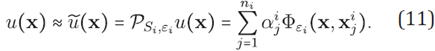
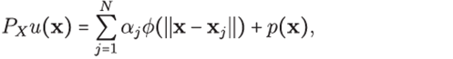
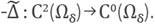
interpolation with Radial Basis Functions the objective is to reconstruct a d-variate function u defined on a bounded domain Ω⊂ℝd from the values u( xk ) of u on a finite set of N scattered points X = {x 1 ;x 2 ; ... ;x N } ⊂Ω⊂ℝd. A radial basis function with shape parameter ε is defined as ɸε:ℝdxℝd→ℝ [6],[31], [34] such that ɸε(x,y)=ɸ(ε||x-y||), where ɸ:(0,∞)→ℝ is an univariate function. A sufficiently smooth function u:ℝd→ℝ can be approximated by the interpolant.
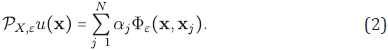
By forcing the condition PX,ε u( xk ) = u( xk ) for k = 1,...,N, the weights αj can be determined by solving the linear system.
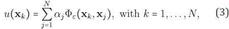
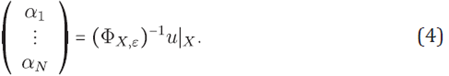
provided that the interpolation matrix ɸX,ε = ɸε( xk ,xk )) 1≤k,j≤N is non-singular and hence the interpolant PX,ε u with
In particular, applying the Gaussian function ɸ(r)=e-r2, the interpolation matrix ɸX,ε is positive definite. Some important results about the convenience and properties of interpolation with this function can be found in [6].
The order of the approximation u(x) ≈ P X,ε u (x) can be measured by the fill distance of X in Ω defined by

and the stability [34] by the separation distance of X defined by
It is worth noting that RBF interpolation is meshless because it can be applied to scattered data with no dependence on point distribution. This property and the values of the shape parameter ε are commonly used to choose a geometry that may improve some performance or relevant aspects of the problem.
GLOBAL COLLOCATION METHOD WITH RBF
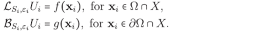
In recent years there has been increasing interest for obtaining approximated solutions of partial differential equations by the collocation method via RBF interpolation, either by unsymmetrical collocation or symmetric collocation [29]. Details for the latter can be consulted in [35]. Next, the unsymmetrical method will be described [19]. Under the RBF interpolation framework, we want to approximate the solution of boundary value problems in the formula
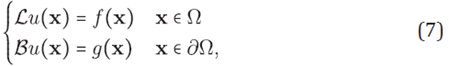
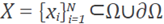
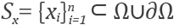
where ℒ and ℬ are linear partial differential operators with regular coefficients have a regularity that is good enough. It is assumed that (7) it is a well-posed problem. Let
 be a set of points conveniently separated as
 and
and
 If it is supposing that the unique solution of (7) can be approximated by the interpolant PX,ε in (2), the problem may be forced by the equations
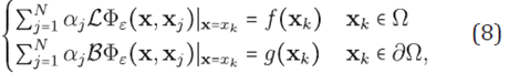
arising from the linear system
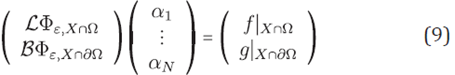
and by (4), obtaining the following linear system whose unknowns are the u values at the points of X
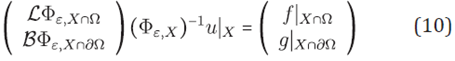
To get the approximated solution u from (10), it is necessary that the collocation matrix (ℒɸε,x∩Ω ℬɸε,X∩∂Ω)t be non-singular, which in general is not true. An elaborated counterexample using multiquadrics and Gaussians was presented in [15]. However, under certain conditions, unsymetrical collocation method is feasible from a generalized approach using separated trial and test spaces [23],[24].
DISCRETIZATION BY RBF-FD
For problems requiring to compute solutions on large domains good resolution, the resultant matrix obtained by the collocation method is dense, huge and ill-conditioned, implying a prohibited computational cost. A variant of RBF collocation method enabling to deal with large domains is the local version [33],[36]. A local interpolation is possible to obtain a sparse matrix that represents the linear partial differential operator. This approach is often called Radial Basis Function-generated Finite Differences method (RBF-FD). The RBF-FD method is the following.
Let
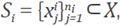
 be a set of interpolation points. For any x
¡ ∈ X an influence domain S
¡ ⊂ X is created which is formed by the n
i nearest neighbor interpolation points. That is, consider an n
i- stencil
be a set of interpolation points. For any x
¡ ∈ X an influence domain S
¡ ⊂ X is created which is formed by the n
i nearest neighbor interpolation points. That is, consider an n
i- stencil
 where
where
 and Ωi = ConvexHull(Si). This is how the subsets
 of points contained in X. u(x) are formed, which be approximated by RBF interpolation for x ∈ S
i as
of points contained in X. u(x) are formed, which be approximated by RBF interpolation for x ∈ S
i as
with x ∈ Ωi. On the shape parameter ε i is on depending on the location xi . This allows to manipulate the shape of the RBF according to known data. Collocating the ni points of the stencil Si , results in a small linear system given by

with
 is the local interpolation matrix and
The unknown coefficients αi in (12) can be expressed in terms of the function values at the local interpolation points as

The inverse matrix
 exists because of the positive definiteness of
 [6]. Now, with the aim of obtaining a local discretized version for (7) consider x
i ∈ Ω∩X or X
i ∈ ∂Ω∩X. In both cases a linear partial differential operator must be applied, either ℒ or ℬ, to equation (11). For xi ∈ Ω it follows
[6]. Now, with the aim of obtaining a local discretized version for (7) consider x
i ∈ Ω∩X or X
i ∈ ∂Ω∩X. In both cases a linear partial differential operator must be applied, either ℒ or ℬ, to equation (11). For xi ∈ Ω it follows
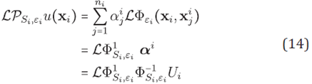
where
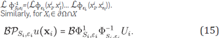
We denote
 and
and
 From (14) and (15) it follows a discretized local version of (7)
The above system of linear equations can be assembled forming sparse matrix H of size N x N where the z-th row, associated to
x¡
∈ X, has at most ni nonzero entries,and the unknown matrix is given by U = ũ(
x1
) ũ(
x2
)...ũ(
xN
) (recall
 ).
).
An approximated solution ũ(x) at all the interpolation points can be obtained by solving HU = F. H can be considered a discretized version of the operator ℒ including the boundary conditions involved in (7). The foregoing discussion gives rise to the following definition.
Definition 1. Let Let ℒ:
Ck
(Ω)→
Ck-m
(Ω) be a linear partial differential operator of order m, where Ω ⊂ ℝ
d
is open and bounded. For u ∈
Ck
(Ω) and x ∈ Ω consider an n−stencil
 of nearest neighbors to x. Here
x1≡x.
The Gaussian RBF-FD operator associated to L denoted by ℒ
Sx
,ε is defined by
of nearest neighbors to x. Here
x1≡x.
The Gaussian RBF-FD operator associated to L denoted by ℒ
Sx
,ε is defined by

Where
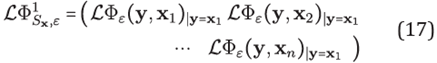
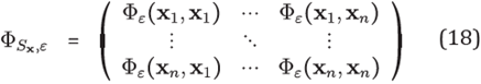

and ɸε( y;xi ) = ℯ−ε2||y−xi||2 with ε > 0. The Gaussian weights matrix of ℒ at Sx is defined by

initially the application of Gaussian RBF-FD implies the solution of a small linear system at every node in order to compute weight matrices, a condition that increases the computational complexity of the problem. There are situations where the non-singular matrix ɸ Sx, ε is ill-conditioned, principally for small values of ε. In these events the RBF is near to the flat limit, however this issue has been overcome by using different methodologies resulting in stable calculations of (20), for example [10]-[12],[22], and recently [26] have used an hybrid kernel that is formed with two weighted terms, one Gaussian and another cubic which is given by '𝜑(r) = αℯ−[εr]2+ βr3 , so this new hybrid kernel now involves three parameters.
Some RBF's do not contain a shape parameter ε. One well known example are polyharmonic splines 𝜑(r) = r 2m log r,m ∈ ℕ and 𝜑(r) = r 2m;m ∉ ℕ. In general a RBF interpolator has the form
where p(x) is a low degree polynomial. The inclusion of p(x), determines the invertibility of the interpolation matrix and this can be explained in terms of the theory of conditionally positive definite functions (for a wider perspective the reader may consult [34],[6]). For example polyharmonic splines include p(x), while the gaussian function does not.
Up to now two kinds of RBF's have been applied in RBF-FD methods (i) infinitely smooth RBF's (which is the approach used in this paper) which contains a shape parameter. In this case is possible to get a high degree of accuracy in the solution although it is necessary to design strategies or algorithms for tuning the best value of the shape parameter and (ii) polyharmonic splines combined with the polynomial term RBF(PHS)- FD for short. This combination is free from a shape parameter but depends on the choice of PHS and polynomial degrees. ɸ(r) is less in uential but p(x) cannot exceed a certain maximum, which increases with the local support size. Thus, the error estimates of RBF(PHS)-FD will depend on knowing the maximal permissible degree of supplementary polynomials (see Fornberg's book [8] for further information).
In this work, to obtain a relatively cheap solver, we focused on obtaining predictable weights with closed formulas depending on ε and h, ε will be adaptable according to the minimum local truncation error at position x. So we will be exploring within small stencils of node sets distributed on regular grids. The node density distribution may cause problems as to accuracy of the method. [8] discuss some methods in quasi-uniform node sets. In order to avoid point sets with sharp density differences we apply the algorithm from [30].
SHAPE PARAMETER FOR SOLUTIONS OF HELMHOLTZ EQUATION
For an homogeneous media the propagation of time-harmonic waves is modeled by Helmholtz equation with wavenumber k = ωc−1 where c is the sound speed and ω is the angular frequency. From the Fourier optics standpoint a time-harmonic wave can be seen as a superposition of plane waves and from the stationary phase method the timeharmonic wave field, at distant points, is due to a plane wave component; therefore it makes sense to consider planes waves as a key part of the analysis. Wave planes are a fundamental tool for investigating the behavior of numerical solutions for Helmholtz equation, either to reduce pollution effects or to design higher order discretizations, in this token, there are recent works such as [18] and [13].
Described below the method to obtain adequate shape parameters on general stencils for approximating a linear dierential operator ℒ with smooth coefficients.
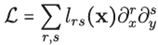
when it is applied to solutions of Helmholtz equation. Let
 be the symbol of the linear differential operator X [37]2. In particular consider plane waves given by
 , therefore u satises

Let
 be an n-stencil with respect to
x1
= x = (x,y). The local truncation error by the approximation ℒ
S,
∈
u(x; k; θ) is given by
be an n-stencil with respect to
x1
= x = (x,y). The local truncation error by the approximation ℒ
S,
∈
u(x; k; θ) is given by
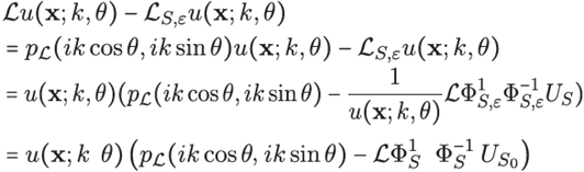
where US0 = (u(x1 − x; k; θ)...u(xn − x; k; θ))t. Note that
In particular, if
 then pℒ(ik cosθ; ik sin θ) = (ik)
r+s
cosr θ sinsθ. Also, since the symbol of Laplace operator is the polynomial pΔ (ξ,Ƞ) = ξ2+ Ƞ2, then pΔ(ik cos θ; ik sin θ) =−
k2
.
then pℒ(ik cosθ; ik sin θ) = (ik)
r+s
cosr θ sinsθ. Also, since the symbol of Laplace operator is the polynomial pΔ (ξ,Ƞ) = ξ2+ Ƞ2, then pΔ(ik cos θ; ik sin θ) =−
k2
.
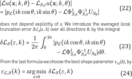
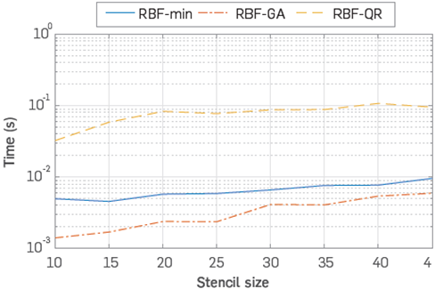
For implementations purposes, we approximated the integral (23) by means of Simpson's rule with ΔΘ=2π/16. To estimate the minimum argument (24) we used the Matlab function fminbnd.m, which use both Golden-section search and parabolic interpolation. This estimate requires roughly range between ten and twenty evaluations of (23). At each iteration, ℒ
 calculated once by Cholesky decomposition. With this procedure we try to reduce dispersion and pollution effects in numerical solutions of Helmholtz equation, calling this algorithm RBF-min.
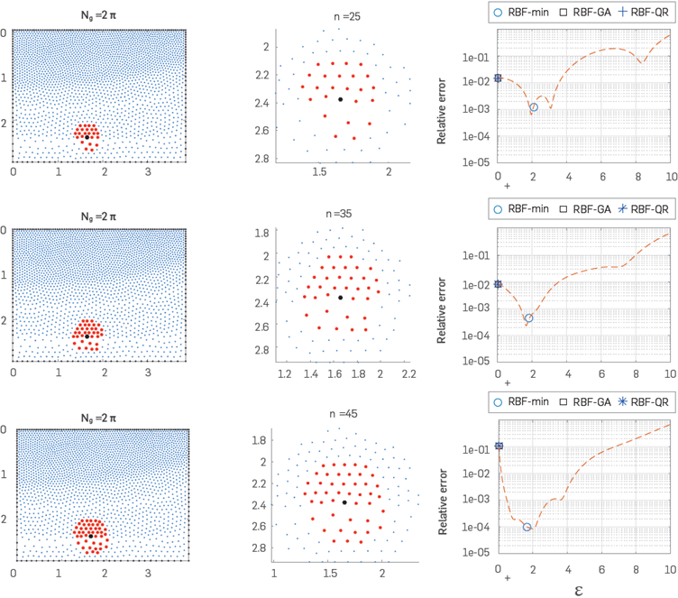

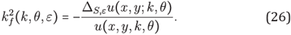
DISPERSION ANALYSIS
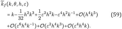
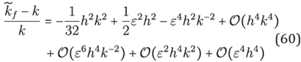
Consider a solution u of Helmholtz equation -Δu(x)-k2u(x)=0. The classical dispersion analysis applies the relative phase error | k-kf |/k where kf is the wavenumber of the numerical solution, which locally satises

The occurrence of the fictitious wavenumber kf is known as numerical dispersion and can be studied by the phase lag | k-kf |. However, as the solution of the Helmholtz equation fluctuates considerably for large wavenumbers the situation is even worse because for measuring the properties of a finite difference scheme, considering only the convergence order is not enough. In fact, the accuracy of the numerical solution deteriorates with increasing wavenumber k even when the resolution factor kh, is kept constant. This phenomenon is related to the so-called 'pollution effect' (see, [17]). Therefore our next task is to build an strategy to mitigate this phenomenon.
To obtain an explicit relation between k and kf we consider the plane wave
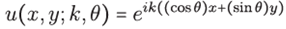
with propagation angle θ and wave length λ=2π/k. According to (25) we can take kf as a function which depends on k, θ the stencil S and ε, given by its square
Note that the local truncation error (22) for ℒ=Δ is given just by

The fictitious wavenumber is anisotropic, i.e., it depends on the wave propagation direction θ. As was the case in [27], our objective will be to choose the shape parameter ε such that the average phase error, over all angles of propagation, is minimum. Hence in minimizing the averaged local truncation error
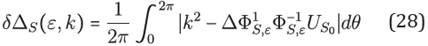
for the variable ε we can mitigate the pollution effect due to dispersion error
SOME CLOSED FORMULAS AND TRUNCATION ERROR
In the context of numerical solutions of the wave equation, numerical stability and isotropy are enhanced with a similar computational work when compared with the standard numerical methods in the simulation of heterogeneous and random media. For example, whereas Von Neumann stability in solution of the 2D acoustic wave equation by explicit finite differences with 5-points needs to satisfy the estimate
 , with hexagonal 7-stencil, this estimate is improved to
 [7]. Besides, with hexagonal stencils we have reached similar results to those reported in [3] where the authors have developed an optimal Cartesian 9-stencil for Helmholtz equation with the goal of mitigating the pollution effect.
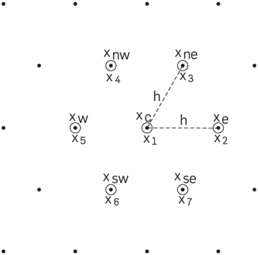
We start considering the 7-stencil
 , built on an hexagonal regular grid as in Figure 3. For h > 0 and
x1
= (x; y) as central node, the coordinates of the other points in H are given by
, built on an hexagonal regular grid as in Figure 3. For h > 0 and
x1
= (x; y) as central node, the coordinates of the other points in H are given by
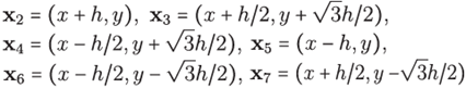
Sometimes will be convenient to work with subscripts referred by cardinal directions:

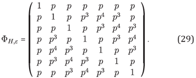
With the given labeled order in the 7-stencil H and with p = ℯ−[εh]2, the interpolation matrix ɸH,ε is explicitly given by
From this formula, we seek expressions for
 and Δ
H
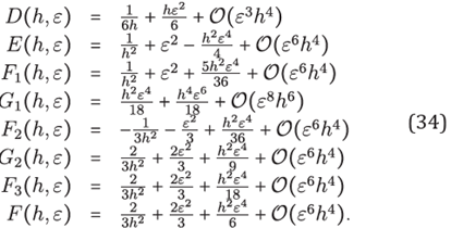
,ε applied at u(x1). Using a software of symbolic calculus we obtain
and Δ
H
,ε applied at u(x1). Using a software of symbolic calculus we obtain
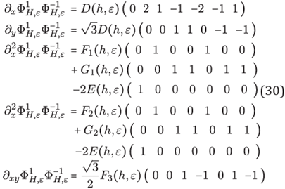
where
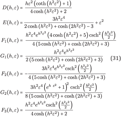
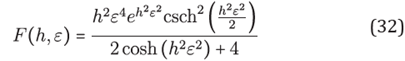
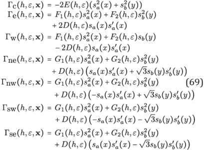
Also, we note that F1 + F2 = G1 + G2 and denote it by F = F1 + F2 = G 1 + G 2, explicitly
Formulas for partial derivative operators of second order. By simple substitutions with the group of equations (31) within of equations in (30) we have explicit formulas for approximating partial derivative operators of second order
As it is usual in finite differences schemes, once an approximation is proposed, the first step is to investigate its local truncation error. The standard methodology consists in making comparisons with Taylor polynomials. The next lemma will be useful in that sense.
Lemma 1. For
 the following approximations of weights functions in (31) hold
One way to test the quality of the method is to point out the relationship with other finite difference schemes. It is not difficult to show that the standard finite difference method is the limit of the RBF-FD scheme, it occurs when the width of the Gaussian RBF, controlled by the shape parameter ε, tends to be at.
Remark 1. By examining the limit situation ε→ 0+ with Δ H,εu (Xc) in (33) via approximations in (34) we recover the formula
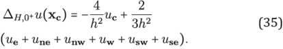
Given in [7], corresponding to the standard finite difference formulation derived by Taylor expansions.
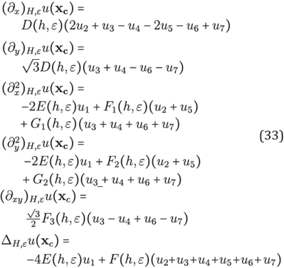
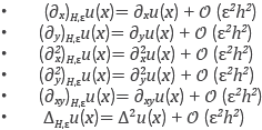
Local truncation errors. To estimate the local truncation error of the approximations ℒ H,εu(x) ≈ ℒu(x) it suffices to expand u(xi), for i = 2, 3; ..., 7 in Taylor polynomials around x1 = xc, and then substituting them in (33), obtaining
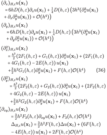
From Taylor polynomials in (34) the following error can be obtained
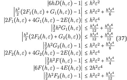
from which the error estimates can be obtained for (33) with their respective approximation errors
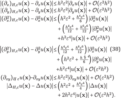
The above treatment and discussion can be summarized in the next result
Theorem 1. Let u be a function in
C4
(Ω) with Ω⊂ℝ2 a convex open set. Then for x ∈Ω , h > 0 small enough such that H⊂ Ω and ε>0 such that
 ; the following assertions about the Gaussian RBF-FD approximations hold:
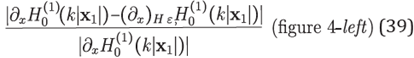
In Figure 4 it is depicted a comparison of RBF-FD with 5-stencils and 7-stencils against its respective standard finite differences approximations. To conduct this test we chose the Hankel function of the rst kind
 with k = 100 and h = 0:01. We can observe the behaviour of the relative truncation error
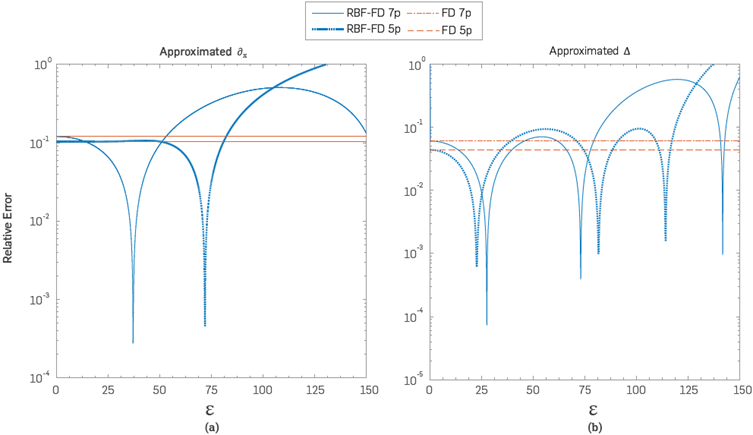
Figure 4 Plot of relative error (left) (39) and (right) (40) with xl = (2; 1:5), k = 100 and h = 0:01
and
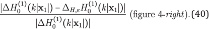
It is worth to point out that in both situations there exist values of ε where the error reaches a minimum value. Furthermore it confirms that the limit situation ε→ 0+, RBF-FD coincides with FD.
OPTIMAL SHAPE PARAMETER ON HEXAGONAL STENCIL
We derive closed formulas to rapidly obtain the optimal shape parameter in the context of hexagonal stencils.
Remark 2. Let u be a solution of the Helmholtz equation. By theorem 1.

for any ε > 0 on a hexagonal stencil H of size h centered at (x;y), we have that for small enough h

In this case the ctitlous wavenumber kf depends also of the stencil size h, kf = kf (k;θ; h; ε) is such that

As we have already seen,
kf\s
related to the truncation error of the Laplace operator applied in u by
In this case, thanks to the symmetry of the hexagonal stencil, it is possible to nd an explicit relation between k and kf. From (33) in (26) we obtain the formula

where
In Figure 5 (left) there is a plot of the residual
 where it can appreciated that for some values of ε It Is possible to have good accuracy even in scaling h for keeping hk = 1 or equlvalently
 that is, by fixing 2π ≈ 6 points per wavelength. Next lemma will allow us to Introduce a simplified variant of (43) which does not depend of θ, by just taking the mean value over [0,2π].
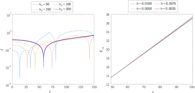
Figure 5 Left: Plot of 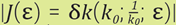 for four different values of
k0
. Right: Plot of ε = ε
op
(100;h) for four different values of h.
for four different values of
k0
. Right: Plot of ε = ε
op
(100;h) for four different values of h.
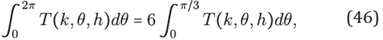
Lemma 2. For any (h,k) ∈ℝ 2, T as in (44) satlses the equality
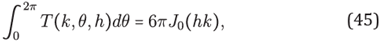
where J 0 is the Bessel function of first kind.
Proof. First, note that
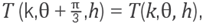 thus T has period
 in the second argument and
then, considering the identity
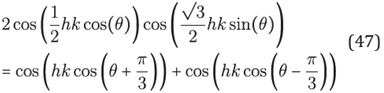
and by a few changes of variable we can finally obtain
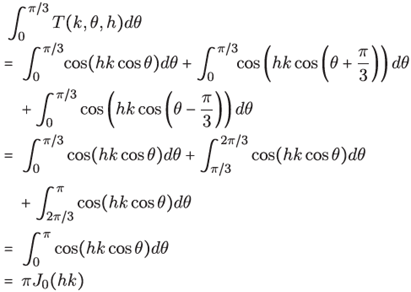
where the last equality is a well known integral representation of the Bessel functions. We define
 such that
explicitly results in the formula

and we also introduced a new residual function
 We will see later what is the error between
kf(k,h,
ε) and
We will see later what is the error between
kf(k,h,
ε) and
 and
and
 produced by "neglecting" θ in taking the mean value (48).
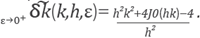
Lemma 3. Let h and k be positive real numbers with small enough h, then
Proof. By supposing
 using the expansions in (34) at (49) and taking ε→ 0+, then lim
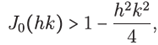
 From the Taylor series of
J0
it is true that
From the Taylor series of
J0
it is true that
and the inequality is thus obtained. For the second limit note that from the explicit formula for (49) given by
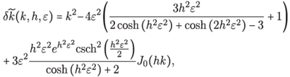
we can see that
In addition, can be observed above that the behavior of
 and
and
 when ε →∞ are the same, hence
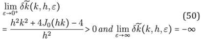
The above lemma and the continuity of the function
 allow us to guarantee that under the condition h > 0 and h > 0 there is some value ε > 0 such that
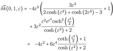
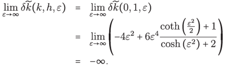
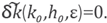
 As we have pointed out, δk measures the dispersion of the approximation, as well δk, thus, given
h0
and k0, a good shape parameter would be ε
0(k0,h0)
such that δ
k(k0,h0,
ε
0
(k0,h0))=0. Our strategy to reduce numerical dispersion is to find the minimum root of the equation
As we have pointed out, δk measures the dispersion of the approximation, as well δk, thus, given
h0
and k0, a good shape parameter would be ε
0(k0,h0)
such that δ
k(k0,h0,
ε
0
(k0,h0))=0. Our strategy to reduce numerical dispersion is to find the minimum root of the equation
 For our implementations we will be more restrictive by considering
 with this we are choosing h so that for sampling a wavelength
 it means to use between 2π to 8π points, that is approximately between 6 and 25 points per wavelength. Thus, in our discretization for the Helmholtz equation on hexagonal stencils we will use the shape parameter

Figure 5 (Right) shows the results of a test focused on behavior of the optimum shape parameter εop. A linear dependence of the wavenumber k is observed; at least in the applied test.
ENHANCED LOCAL TRUNCATION ERROR
This section presents the results of a couple of tests intended to show the order of the local truncation error |Δ
H
,ε
opu
(x)-Δu(x)| and |(∂x)
H
,ε
opu
(x)-(∂x)u(x)|. In Figure 6 shows the results of testing the approximations by comparing with standard FD for u(x)= ℯik-x. Whereas in Figure 7 the same is done with
 Both functions are solutions of the Helmholtz equation, it can be noted that in these cases the optimum shape parameter oers an error of the order (h4).
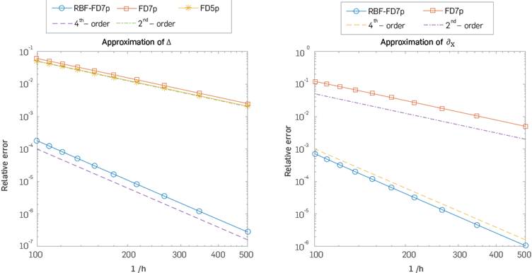
Figure 6 Left: Comparison of relative local truncation error, varying h, between the approximation using standard FD 7p Δ H,0u (x,y) and RBF-FD7p Δ H,0u (x,y). Right: Comparison of relative local truncation error between the approximation using standard FD7p (∂ x ) H,0u (x,y) and RBF-FD7p (∂ x ) H,0u (x,y). Here u(x,y)=ℯik[z cosθ+y sinθ], is evaluated at (x,y)=(2.15), with θ= π|6 and k=100.
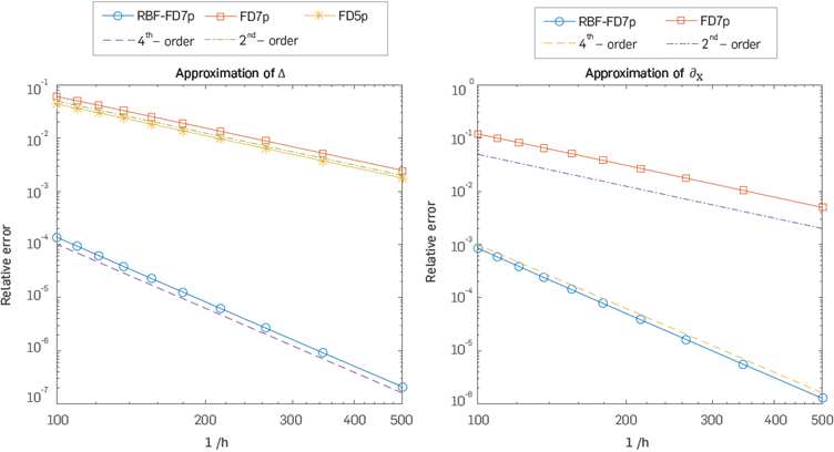
Figure 7 Left: Comparison of relative local truncation error, varying h, between the approximation using standard FD 7p Δ
hu
(x,y) and RBF-FD7p (Δ)
H,ε u
(x,y). Right: Comparison of relative local truncation error between the approximation using standard FD7p (∂
x
)
hu
(x,y) and RBF-FD7p (∂
x
)
H,
εu(x,y). Here 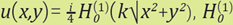 is the Hankel function evaluated at (x, y) = (2, 1:5) and k = 100.
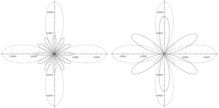
Figure 8 Comparison between the function 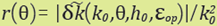 (solid line) where
k0=
100 and h0=0.01, and the function
(solid line) where
k0=
100 and h0=0.01, and the function  (dashed line) where J
ᵧ and parameters b0, d0, e0 and G0 were taken from [3]. Left: εop satises δk(l00,0.001, ε
op)=0. Right:
ε
op= arg min
.
(dashed line) where J
ᵧ and parameters b0, d0, e0 and G0 were taken from [3]. Left: εop satises δk(l00,0.001, ε
op)=0. Right:
ε
op= arg min
.
RELATIVE PHASE ERROR - POLLUTION EFFECT
As is well known through the vast literature about numerical solutions of Helmholtz equation, k is a key parameter. For large values of k, the solution u is highly fluctuating. To approximate the Helmholtz equation with an acceptable accuracy, the resolution of the discretization for the domain of interest should be adjusted to the wave number according to the so called rule of thumb [17],
which prescribes a minimum number of elements per wavelength. However, the performance of standard finite difference or finite element methods, such as the classical Galerkin finite element method, deteriorates as k increases. This misbehavior, known as pollution of the approximate solution, can only be avoided, with standard methods, after a drastic renement of the discretization. [9] summarized the local truncation error
 and the relative phase error (kf,k)l k of the most popular methods for solving Helmholtz equation using different size stencils.
Now our aim isto calculate the approximation order of the numerical wavenumber
 as k changes, in order to estimate the order of the relative phase error, but first we will examine the order of the error
 produced by neglecting the dependence of θ in taking the average value of
on [0.2π]. We recall that
produced by neglecting the dependence of θ in taking the average value of
on [0.2π]. We recall that

and

From the Taylor polynomials of (44) and Bessel function respectively
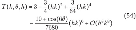
and
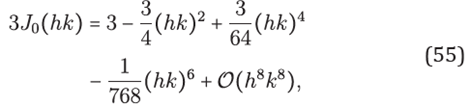
thus
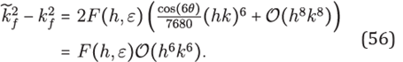
From the approximations of F(h,ε) given in (34), it is easy to

Hence
 On the other hand, from (34), (55)
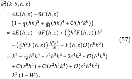
where
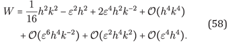
Provided that lWl < 1, the binomial series can be applied, that is
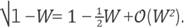 We take the linear approximation, then
Hence the relative phase error is given by
Note that for the limit case ε →0+

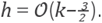
which asserts that, in the limit case, for keeping the order of the error when k is increasing, the mesh size h it must scale at least as
 that is
3. EXPERIMENTAL DEVELOPMENT
Perfectly matched layers (PML) is a technique for simulating solutions of wave phenomena in free-space. The idea is to build an absorbing layer for surrounding the computational domain of nterest. The new system possesses the property of generating no reflection, at least in continuous case, at the interface between the free medium and the articial absorbing medium. PML has been ntroduced by Berenger [1] for Maxwell's equations, and has been widely used for the simulation of time dependent seismic waves as well as Helmholtz-like equations. The analysis necessary to show that the Helmholtz equation with PML (PML-Helmholz) for constant wavenumber is a well-posed problem is treated in [20] Now a description of PML-Helmholtz equation is given (see [14] [38] for details).
For setting up the PML-Helmholtz equation it is necessary to define some basic functions in a rectangular domain. Let σl ℝ→ℝ be defined by
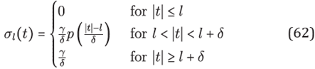
where p (0,1) → (0,1) is given by
 γ and δ are constant. By definition σ ∈C∞(ℝ). for a fixed positive angular frequency ω satisfying
 , let dl be the complex-valued function
Consider the open rectangles Ω=(-a,a)x(-b,b) and Ωδ=(-a-δ,a+δ) x(-b-δ,b+δ).
The modified PML-Laplace operator is defined by
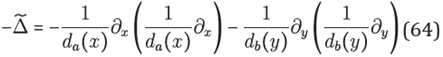
or alternatively
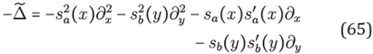
where
 and
and
 Note that
 coincides with -Δ in Ω. Usually, for making analytic studies this is considered as an unbounded operator on
L2(
ℝ2
) with domain the Sobolev space
H2(
ℝ2
) or in a weaker form, as an unbounded operator on H-1(ℝ2) with domain HJ(ℝ2) [38]. However, for numerical implementations in__ the finite difference approach it is considered a truncated version
coincides with -Δ in Ω. Usually, for making analytic studies this is considered as an unbounded operator on
L2(
ℝ2
) with domain the Sobolev space
H2(
ℝ2
) or in a weaker form, as an unbounded operator on H-1(ℝ2) with domain HJ(ℝ2) [38]. However, for numerical implementations in__ the finite difference approach it is considered a truncated version
 The PML-Laplace operator allows to introduce the PML-Helmholtz equation
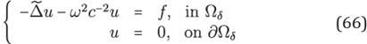
we will suppose that the function c = c(x) which describe the acoustic or P-wave propagation speed is positive and belongs to C2(Ωδ).
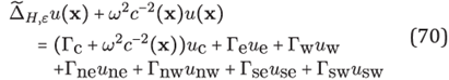
In order to approximate solutions of equation (66) within the approach of RBF-FD on hexagonal grid, we use the explicit expressions for Gaussian weights, thus by way of the formulas in (33) we have that for x = (x, y) in Ωδ with 7-stencil H ⊂ Ωδ
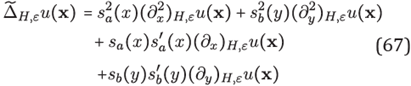
hence by carrying out substitutions
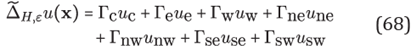
where weights Γ's are given by
and of course,
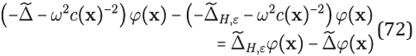
We use the optimal shape parameter ε given by (51) to approximate each operator involved in (68). To analyze the approximation
 applied to problem (66) we regard the concept of consistency [32],
Definition 2. Given a partial differential equation, ℒu = f, and a finite difference scheme, ℒ hu = f based on a stencil with size h, we say that the finite difference scheme is consistent with the partial differential equation if for any smooth function 𝜑(x)

as h → 0, the convergence being pointwise convergence at each point x.
Proposition 1. The RBF-FD approximation given in (67) applied to the problem (66) is consistent with the Helmholtz-PML equation and has second order of accuracy.
Proof. We need to show that for an hexagonal 7-stencil H of size h centered at x ∈Ωδ and for a given shape parameter ε
converges pointwise to 0 as h → 0, where 𝜑 is a smooth function. The proof will be completed by simply inspecting the estimates in (38) used in (67), once performed these substitutions we can observe that

which means that the accuracy of the approximation is 𝒪(ε 2h2 ), as εh tends to 0.
DISCRETE FORMULATION
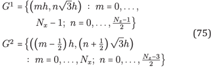
We will perform the discretization of the problem (66) on an hexagonal grid G which represents to ÍÍ6. The optimal shape parameter at every stencil will be taken in accord to its dependence of the local wavenumber k(x) = ω 2c−2 (x), so ε op (x) = ε op (k(x),h), where is used (51). For the sake of a more simplied notation, we denote similarly for the others weights formulas in (69).

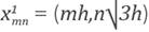
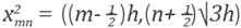
We begin by considering two rectangular grids given by
where
Nz
is a positive odd integer. Note that the grid
G = G1
∪
G2
is formed by hexagonal stencils. We denote
 and
and
 for points in
G1
and
G2
respectively; also we denote
for points in
G1
and
G2
respectively; also we denote
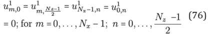
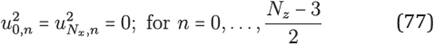
 The homogeneous Dirichlet boundary condition it is expressed in terms of the boundary points of the grid G, by doing
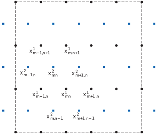
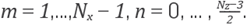
Thus, for points in the grid G1, the equation (68) has the explicit form
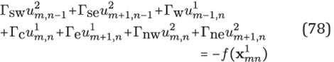
for
 and for points at grid
G2
is
and for points at grid
G2
is
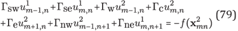
for
 With the couple of equations above we assemble a sparse linear system
 where c is a diagonal matrix formed with the values
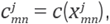
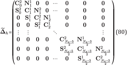
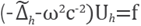
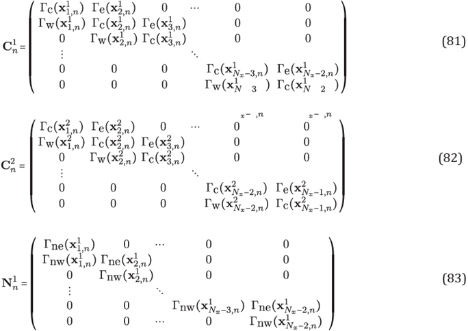
is a block matrix whose blocks are given by
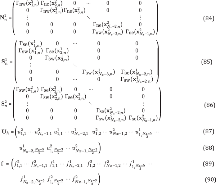
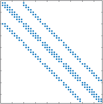
The sparsity pattern of the matrix
 is depicted in Figure 11.
Remark 3. If
 the linear system
LhUh=f can
be solved if only if
the linear system
LhUh=f can
be solved if only if
 Here Σ (A) denotes the spectrum of A. Is pending for a further work to prove that
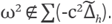
Figure 10 shows a plot of some eigenvalues of the matrices
Here Σ (A) denotes the spectrum of A. Is pending for a further work to prove that
Figure 10 shows a plot of some eigenvalues of the matrices
 and
and
 where c represents the Marmousi model extended to PML. The eigenvalues plotted are 500 nearest to ω2 and 500 nearest to 0.
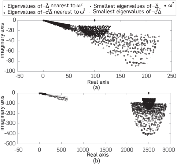
Figure 10 Plot of some eigenvalues of the matrices  and
and  (Top) for ω = 10 and h= 0.1497, (below) ω = 50 and h = 0.0300. c represents the Marmousi model extended to PML.
4. RESULTS
PLANE WAVES
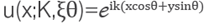
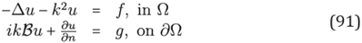
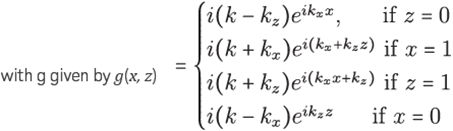
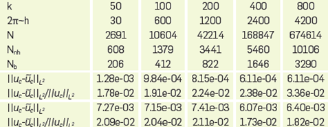
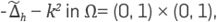
With Ω = (0,1) × (0,1), k = 500, kx = k cos θ, kz = k sin θ . By using 2π points per wavelength, i.e. kh = 1, we solve (91)
SPHERICAL WAVEFRONT
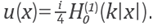
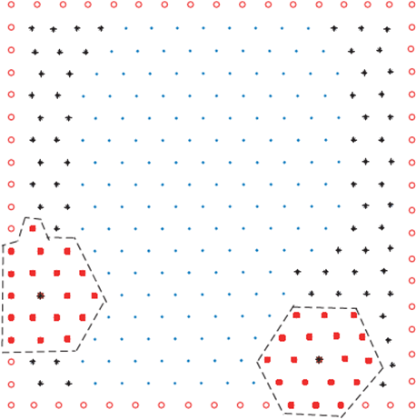
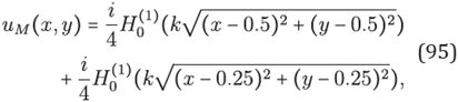
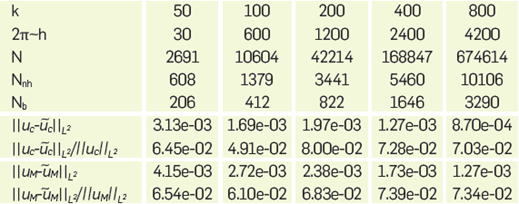
For this example it is chosen Ng = 6 for solving the problem (91) with Ω = (0, 1)x(0,1). Where g is the boundary data satisfying the exact solutions

and
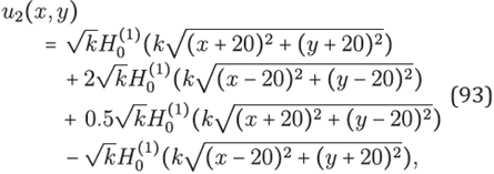
with constant k. These solutions corresponds to a single source and four sources, respectively, outside the domain Ω The relevancy of taking u2 can be seen In [13]. Discretizations were made with Ng = 6 nodes per wavelength at each value of the wavenumber k. Within an hexagonal grid we take 7-stencils at Inner nodes and 22-stencils at boundary nodes.


INSIDE SOURCE PROBLEM
Now we test our method with sources inside the domain. The aim is to get the truncated solution of the problem
WITH PML
In this test we solve the problem of nd the truncated Green's function for
 that is the solution of
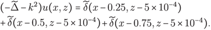
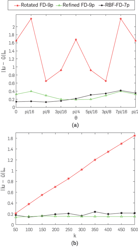
Figure 13 Comparison of results between RBF-FD and those reported in [3]. (a) Results for k = 500 and h = 1/500 varying the propagation angle, (b) With k varying, θ=π/4 and h=1/k
The solution of this problem is
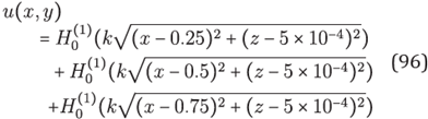
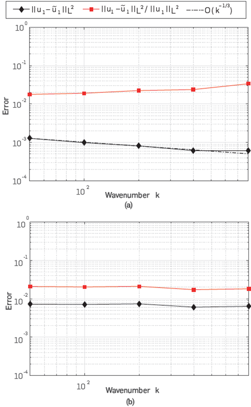
Figure 14 Plot of tests for approximated solutions of (91). (a) Comparison with the exact solution (92). (b) Comparison with the exact solution (93).
where
 is the Hankel function. For this test we use 2π points per wavelength (i.e. kh = 1). Some results with a qualitative analysis of error are shown in Figure 15.
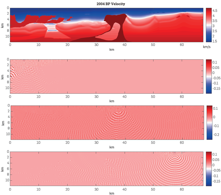
2004 BP MODEL
In this example we calculate the truncated Green function for the well known BP model in frequencies 15Hz and 40Hz. The results are shown in Figure 16.
CONCLUSIONS
In this paper we have developed and applied a RBF-FD method on hexagonal grids that solves the Helmholtz equation for a wide range of values of the wavenumber k We focus in obtaining accurate local approximations of the partial derivative operators by using a few degrees of freedom applied to solutions of Helmholtz equation.
We obtain closed formulas for the weights in terms of ε,h showing that the standard finite difference method is the limit of our RBF-FD scheme, this happens when the wide of the Gaussian RBF, controlled by the shape parameter ε, tends to be flat. The method obtains banded matrices; such that the respective linear systems can be solved efficiently by direct solvers.
We have developed a simple solver that is compared with 5-point Finite difference method and accurate compared with 9-point FD method. By local interpolation we found good shape parameters to approximate derivatives of solutions of the 2D Helmholtz equation. Within the RBF-FD framework are approximated the solutions of the PMLHelmholtz equation on hexagonal grids with optimal values of the shape parameter.
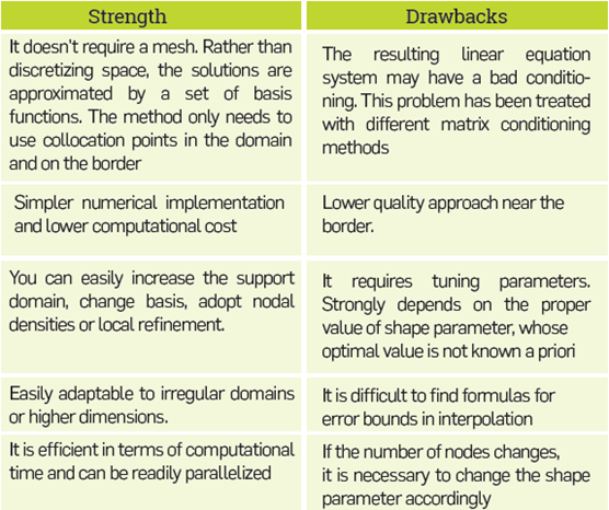
Our method has been compared against classical and well-known methods, showing equal and sometimes better performance, with this we have validated numerically that our solver suer less of the pollution effects. The advantages and drawbacks of the RBF-FD method applied to Helmholtz equation can be seen at Table 3.