Inglés (pdf)
 Articulo en XML
 Referencias del artículo
 Enviar articulo por email
 Citado por SciELO
  Citado por Google
  Similares en
SciELO
Similares en
SciELO  Similares en Google
 Permalink
Introduction
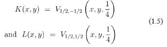
The Voigt functions K (x; y) and L (x; y) are effective tools for solving a wide variety of problems in probability, statistical communication theory, astrophysical spectroscopy, emission, absorption and transfer of radiation in heated atmosphere, plasma dispersion, neutron reactions and indeed in the several diverse field of physics and engineering associated with multi-dimensional analysis of spectral harmonics. The Voigt functions are natural consequences of the well-known Hankel transforms, Fourier transforms and Mellin transforms, resulting in connections with the special functions. Many mathematicians and physicists have contributed to a better understanding of these functions.For a number of generalizations of Voigt functions, we refer Yang (1994). Pathan, et al. (2003), (2006), Klusch (1991) and Srivastava, et al. (1998). Following the work of Srivastava, et al. (1987), Klusch (1991) has given a generalization of the Voigt functions in the form
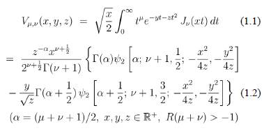
where ψ2 denotes one of Humbert's confluent hypergeometric function of two variables, defined by Srivastava, et al. (1984), p.59
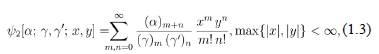
(λ)n being the Pochhammer symbol defined (for λ Ε C) by
The classical Bessel function J v (x) is defined by (see, Andrews, et al. (1999)).
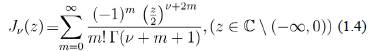
so that
Observe that J v (z) is the defining oscillatory kernel of Hankel's integral transform
p F q is the generalized hypergeometric series defined by (see, Andrews, et al. (1999)).
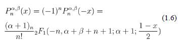
The following hypergeometric representation for the Jacobi polynomials
 is a special case of the above generalized hypergeometric series
Another special case [Prudnikov, et al. (1986), p.579 (18)] expressible in terms of hypergeometric function is
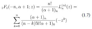
where
 is Laguerre polynomial [Andrews, et al. (1999)].
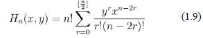
The generalized Hermite polynomials (known as Gould-Hopper polynomials)
 [Gould, et al. (1962)] defined by
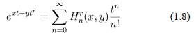
are 2-variable Kampe de Feriet generalization of the Hermite polynomials Dattoli, et al. (2003) and Gould, et al. (1962)
These polynomials usually defined by the generating function
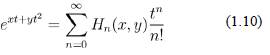
reduce to the ordinary Hermite polynomials H n (x) (when y = -1 and x is replaced by 2x).
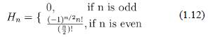
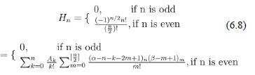
We recall that the Hermite numbers H n are the values of the Hermite polynomials H n (x) at zero argument that is H n (0) = 0. A closed formula for Hn is given by
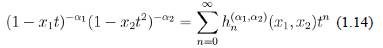
Altin, et al. (2006) presented a multivariable extension of the so called Lagrange-Hermite polynomials generated by [see Altin, et al. (2006), p.239, Eq.(1.2)] and Chan, et al. (2001):
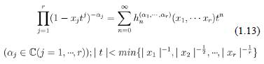
Where
The special case when r = 2 in (1.13) is essentially a case which corresponds to the familiar (two-variable) Lagrange-Hermite polynomials
 considered by Dattoli, et al (2003)
The present work is inspired by the frequent requirements of various properties of Voigt functions in the analysis of certain applied problems. In the present paper it will be shown that generalized Voigt function is expressible in terms of a combination of Kampe de Feriet's functions. We also give further generalizations (involving multivariables) of Voigt functions in terms of series and integrals which are specially useful when the parameters take on special values. The results of multivariable Hermite polynomials are used with a view to obtaining explicit representations of generalized Voigt functions. Our aim is to further introduce two more generalizations of (1.1) and another interesting explicit representation of (1.1) in terms of Kampe de Feriet series
 [see (Srivastava, et al. (1984), p.63)]. Finally we discuss some useful consequences of Lagarange-Hermite polynomials and analyze the relations among different generalized Voigt functions.
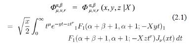
Generalized Voigt function Φ α,β µ,v,r
In an attempt to generalize (1.1), we first investigate here the generalized Voigt function

Denition The generalized Voigt function
 is defined by the Hankel transform
where
 .
.
A fairly wide variety of Voigt functions can be represented in terms of the special cases of (2.1).We list below some cases.
The generalized Voigt function
is defined by the integral representation
where
 .
.
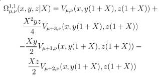
An obvious special case of (2.1) occurs when we take r = 2 and X = 1.We thus have
Clearly, the case X = 0 in (2.1) reduces to a generalization of (1.1) in the form
and (2.2) corresponds to (1.1) and (1.2) and we have
And
Moreover,
 is the classical Laplace transform of t
u
J
v
(xt). The case when z = 1/4 and X = 0 in (2.1) yields
is the classical Laplace transform of t
u
J
v
(xt). The case when z = 1/4 and X = 0 in (2.1) yields
Using the denition (2.1) with α = 0, β = 1 and applying [Prudnikov, et al. (1986), p.581(35)]
we get a connection between
 in the form
where Vμ,V is given by (1.1).
Similarly setting α = 1, β = 1 and applying [Prudnikov, et al. (1986), p.582(53)]
we get
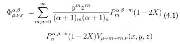
Explicit Representations for Φ α,β µ,v,r
In (2.1),we expand 1 F' s 1 in series and integrate term. We thus find that
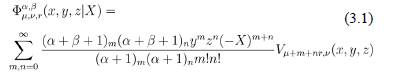
which may be rewritten in the form
where we have used the series manipulation [Srivastava, et al. (1984), p.101(5)]
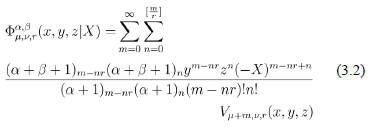
By using a well-known Kummer's theorem [Prudnikov, et al. (1986), p.579(2)]
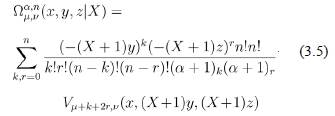
in (2.1) yields
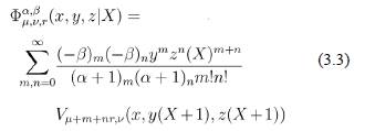
which further for X = 1 and r = 2 reduces to
For r = 2, (3.3) reduces to the representation
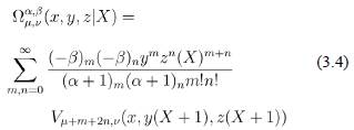
In view of the result (1.7)[Prudnikov, et al. (1986), p.579(18)] with β = n (n an integer),(3.4) reduces to
Series expansions of Ω α,β µ,v,r involving Jacobi, Laguerre and Hermite polynomials
We consider the formula [Srivastava, et al. (1984), p.22] expressible in terms of Jacobi polynomials
 (x)[2] in the form
which on replacing t by yt and t by zt r gives
And
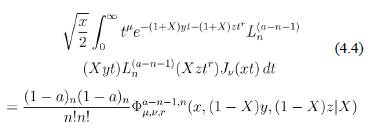
respectively. These last two results are now applied to (2.1) to yield a double series representation
As before, set r = 2 and use
 to get
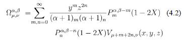
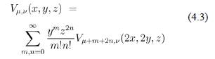
Putting X=0 and using the property
 in (4.2),we obtain the following representation
Now consider a result [Prudnikov, et al. (1986), p.579 (8)] connecting 1F1 and Laguerre polynomial
which on replacing t by yt and t by zt r gives
And
respectively. These last two results are now applied to (2.1) to yield an integral representation
The use of generalized Hermite polynomials defined by (1.8) can be exploited to obtain the series representations of (2.1). We have indeed
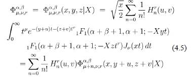
by applying (1.8) to the integral on the right of (2.1). Since
we may write a limiting case of (2.1) in the form
which further for X=0 reduces to
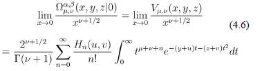
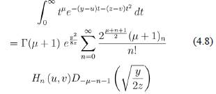
Now in (4.6), using [Erdelyi, et al. (1954), 146(24)]
where D. v (x) is parabolic cylinder function [Prudnikov, et al. (1986)], we have
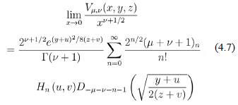
A reduction of interest involves the case of replacing y by y -u, z by z - v and μ by μ - v, and we obtain a known result of Pathan and Shahwan [10] (for m=2) in its correct form
Connections
We consider the following two integrals
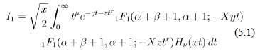
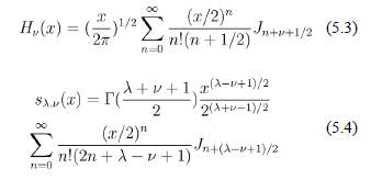
where Hv (x) are Struve functions [Luke (1969), p.55(8)], x, y
 .
.
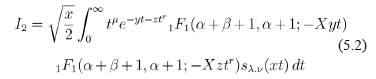
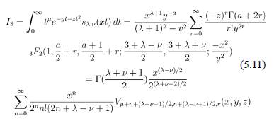
where sλ,v (x) are Lommel functions [Luke (1969), p.54 (9.4.5) (3)],
 .
.
To evaluate these two integrals,we will apply the following two results [Luke (1969), p.55(8)] and [Luke (1969), p.54(9.4.5)(3)]
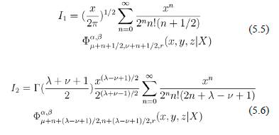
Making appropriate substitution of Hv (x) and Sλν (x) from these two results in (5.1) and (5.2), we get
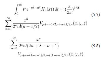
For X=0, (5.1) and (5.2) reduce to
Setting r=2 and z = 1/4 in (5.7) and comparing with a known result of [Pathan, et al. (2006), p.78(2.3)], we get
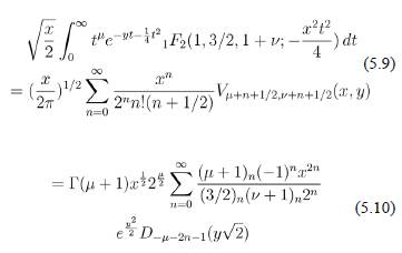
Setting r=2 in (5.8) and using [Prudnikov, et al. (1986), p.108], we are led to another possibility of dening the Voigt function in the form of Appell function. Thus we have
where α = λ + μ + 1.
Voigt function and numbers
First we consider a number which we denote by A k with a generating function
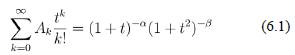
The series expansion for A k is
On comparing (6.1) with (1.14),we find that the number Ak and Lagrange-Hermite numbers are related as
Moreover from (6.1),we can obtain the following two Laplace transforms
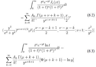
where Ψ is logarithmic derivative of Γ function [Andrews, et al. (1999)].
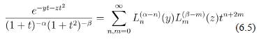
Now we start with a result [Srivastava, et al. (1984), p.84 (15)] for Laguerre polynomials
which on replacing t by t2, α by β and y by z gives
On multiplying these two results yields
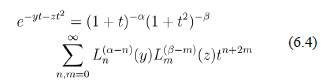
which is equivalent to
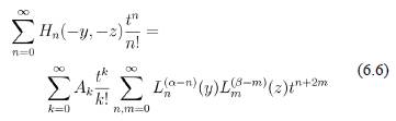
Using (6.1) and (1.10) in (6.4) gives
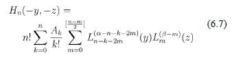
Comparing the coecients of t n on both the sides of (6.6), we get the the following representation of Hermite polynomials in the form
In view of the result (1.12) expressed for Hermite numbers Hn, for y = z = 0,(6.7) gives
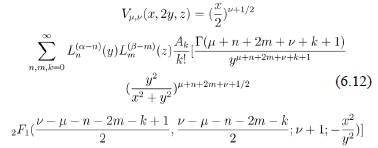
Now we turn to the derivation of the representation of voigt function from (6.7). Multiply both he sides of (6.4) by
 and integrate with respect to t from 0 to ∞ to get
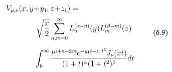
which on using (6.1) gives
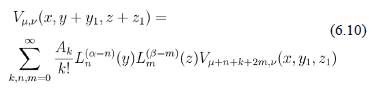
For y = z = 0, (6.9) gives an interesting relation between Voigt functions in the form
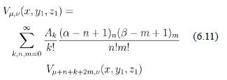
Yet, another immediate consequence of (6.9) is obtained by taking y1 = y = z1 = 0 and applying (6.2). Thus we have
By setting z=0 in (6.4) and multiplying both he sides by
 ln t, integrating with respect to t from 0 to ∞ and using (6.3) and [Erdelyi, et al. (1954), p.148(4)]
we get
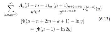
where Ψ is logarithmic derivative of Γ function [Srivastava, et al. (1984)].
If, in (6.5),we set α = β = 1, multiply both he sides by
 and integrate with respect to t from 0 to ∞, we get a generalization of (6.10) in the form
Some useful consequences of Lagarange-Hermite polynomials.
Now we start with a result [Srivastava, et al. (1984), p.84 (15)] for Laguerre polynomials written in a slightly different form
which on replacing t by t2, α by β, x1 by x1 and y by z gives
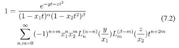
On multiplying these two results and adjusting the variables yields
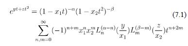
which is equivalent to
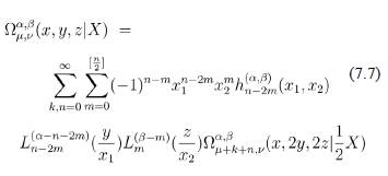
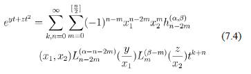
Using the definition of Lagrange-Hermite polynomials
 given by (1.14) in (7.2), we get
which on replacing n by n-2m gives
Again applying the denition of Hermite polynomials given by (1.10) in (7.4), replacing n by n-k and comparing the coecients of t n , we get the following representation of
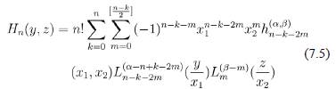
which reduces to (6.7) when we take x1 = x2 = 1 and use A
k
=
 .
.
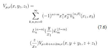
It is also fairly straightforward to get a representation of generalized Voigt function V
μν by appealing (7.3). We multiply both he sides by fe
-
 and integrate with respect to t from 0 to ∞. Thus we get
On the other hand, multiplying both the sides of (7.4) by
and integrating with respect to t from 0 to ∞and then using (2.2), we get a generalization of (6.10) in the form