


Servicios Personalizados
Revista
Articulo
 Inglés (pdf)
 Articulo en XML
 Referencias del artículo
 Enviar articulo por email
Indicadores
-
 Citado por SciELO
 -
 Accesos
Links relacionados
-
 Citado por Google
 -
 Similares en
SciELO
Similares en
SciELO -
 Similares en Google
Compartir

 Permalink
Revista de Economía del Caribe
versión impresa ISSN 2011-2106
rev. econ. Caribe no.9 Barranquilla ene./jun. 2012
ARTÍCULO DE INVESTIGACIÓN
Bio-Fuel Market: Hypothetical Scenarios
El mercado de bio-combustible: Escenarios hipoteticos
Juan M. Dominguez*
Ph. D. ESPAE-Graduate School of Management/Center for Renewable and Alternative Energy. Escuela Superior Politecnica del Litoral (ESPOL), Guayaquil-Ecuador. jdomingu@espol.edu.ee
I would like to thank the participants of the Ph.D. Seminar at the University of Minnesota for their invaluable comments. I would also like to thank to my Research Assistant, Sharon Guaman, for her invaluable help in editing this document. All remaining errors are those of the author.
Fecha de recepcion: noviembre de 2011
Fecha de aceptacion: febrero de 2012
ABSTRACT
This paper employs the Ivaldi-Vibes algorithm to model the U.S. fuel market under the hypothetical scenario in which the ethanol production subsidies were phased out from 1995- 2005. Under this hypothetical situation, the individuals were not only willing to switch their consumption decision, but they were also willing to consider alternative modes of transportation including public transportation, biking or walking. As a result, the outside alternative market share increased about 4% and 6% and the conventional fuel market shares increased while the ethanol blends experienced decreases across all petroleum districts.This methodology also permitted simulating the impact of this elimination on the fuel prices. The conventional fuel prices increased in a range between 0.12 and 1.34 percent. Finally, since different types of oxygenates are blended with the regular fuel to compliance the EPA regulations, the reduction in the reformulated gasoline market shares implied a trade off in the demand for these oxygenates whose variation rates averaged 55.14% for the ethanol-MTBE ratio.
Palabras clave: Biofuels, ethanol, production subsidies, oxygenates, marginal costs.
Clasificacion Jel: Q16, H23,H25,Q52.
RESUMEN
En este trabajo se emplea el algoritmo de Ivaldi-Vibes para modelar el mercado de combustibles de EE.UU. bajo el escenario hipotetico en el que los subsidios a la production de etanol fueron eliminados desde 1995 hasta 2005. En esta situation hipotetica, los individuos no solo estaban dispuestos a cambiar su decision de consumo, sino tambien a considerar modos alternativos de transporte, incluyendo el transporte publico, en bicicleta o caminar. Como resultado, la cuota de mercado exterior alternativa aumento un 4% y 6% y las cuotas del mercado de combustibles convencionales aumento, mientras que el etanol combinado experimento disminuciones en todos los distritos petroleros. Esta metodologia tambien permite simular el impacto de esta elimination en los precios de los combustibles. Los precios de los combustibles convencionales aumentaron en un rango entre 0,12 y 1,34 por ciento. Por ultimo, ya que los diferentes tipos de compuestos oxigenados son combinados con la gasolina regular para el cumplimiento de las regulaciones de la EPA, la reduccion de las cuotas de mercado de combustibles reformulados implica un trade-off de la demanda de estos productos oxigenados, cuya tasa de variacion promedio es de 55,14% para la razon etanol- MTBE.
Keywords: Biocombustibles, etanol, subsidios a la production, oxigenados, costos marginales.
Jel codes: Q16, H23,H25,Q52. [2]
1. INTRODUCTION
Interest in issues related to the environment and energy security at world-wide level has increased over the past decade. Those factors along with the incentives to use agricultural commodities to produce industrial products and increases in the petroleum prices have motivated the development of alternative fuels such as ethanol, biodiesel and natural gas.
In the United States, specifically, there are two major renewable fuels that are being produced: ethanol produced from grain, and biodiesel produced from vegetable oils and animal fats. Indeed, the demand for ethanol and biodiesel is mostly mandated by federal and state legislations.
According to the study done by Koplow (2006), subsidies in the ethanol industry have a long tradition which started with the EnergyTax Act of 1978 that introduced the first federal subsidization of ethanol production. That Act established a full exemption of 0.04US$/gallon motor fuel excise tax1 for ethanol-gasoline blends. The Energy Security Act of 1980 and the Crude Oil Wind- fall Profits Tax Act of 1980 provided federally-insured loans for ethanol producers and extended the ethanol-gasoline tax exemption through the end of 1992. It is worth noting that the former Act allowed guarantees of up to 90% of the construction cost for production capacities of less than one million gallons a year2. In 1980 a tariff of 0.50 US$/ gallon was also introduced in order to protect the domestic production of ethanol. This tariff was increased 0.60 US$/gallon with the implementation of the Deficit Reduction Act of 1984. Furthermore, these incentives were not only directed to the producer's side, but also a federal legislation encouraged consumption side through the Alternative Motor Fuels Act of 1988 which provided credits to automakers that satisfied their Corporate Average Fuel Economy standards for car fueled by alternatives fuels.
The Clean Air Act Amendments (CAAA) of 1990, the Energy Policy Act of 1992, and the Energy Conservation Reauthorization Act of 1998 allowed the growth of the renewable fuel industry during the 1990s. Recently, the Farm Security and Rural Investment Act of 2002, American Jobs Creation Act 2004 and the Energy Policy Act of 2005 have strengthened the development of these biofuels. The following table presents a brief summary of the federal policies of the blenders' credits that have contributed to the development of the biofuel industry:
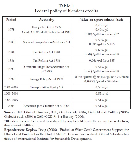
It is worth mentioning that the current tariff is about 0.54 US$/gallon and that the Energy Policy Act of 2005 established a minimum consumption level for biofuels called the Renewable Fuel Standards (RFS). RFS mandates the purchase of four billion gallons of renewable fuels in 2006, increasing to 7.5 billion in 2012 with increases equivalent to the increase in gasoline after that.
The Clean Air Act Amendments (CAAA) of 1990 established two major oxygenate requirements in order to address two specific air-pollution problems. An oxygenate was required to be blended to reformulated gasoline and oxygenated fuels. In the past, the methyl tertiary butyl ether (MTBE) was the main oxygenate utilized by refineries. Ethanol and MTBE were considered substitutes for this end use, but MTBE is currently being phased out in most of the states due to potential groundwater contamination. The MTBE bans have certainly affected the demand for ethanol guaranteeing it a market share as the most important oxygenate.
The oxygen content requirement included in the federal and state policies and regulations has opened a market for ethanol fuel3. As I previously mentioned, there are, in fact, some blended products derived such as the reformulated gasoline4 (RFG), E10 (fuel composed of 10% of ethanol, 90% of gasoline) and E85 (fuel composed of 85% of ethanol, 15% of gasoline). The last two products could be grouped into the category of oxygenated gasoline because of their minimum oxygen requirement which is at least 2.7%. However, there exists skepticism to consider ethanol and the derived products as possible substitutes for the conventional gasoline due to the fact that ethanol competitiveness is mostly based on the subsidies established to promote the development of clean fuel alternatives. Moreover, there are technical concerns such as its low energy content and the logistics involved in the distribution of these biofuels.
It should be noted that the Environmental Protection Agency (EPA) is amending the RFG regulations and all provisions which were included to ensure compliance with the oxygen content requirement. There are two rules, called the Direct Final Rules (DFRs),that amend the RFG regulations to remove the oxygen content requirement because the Energy Act provided for different compliances date for the removal of the RFG oxygen requirement in California and the rest of the country. These rules also revise the current prohibition against commingling VOC5-controlled RFG blended with ethanol with VOC-controlled RFG with any other type of oxygenate. This revision is also to prohibit combining VOC-controlled RFG blended with ethanol with non-oxygenated VOC-controlled RFG except under certain limited circumstances. These two DFRs have become effective on April 24 and May 5, 2006 for California and gasoline nationwide respectively.
Even though there will no longer be an oxygen content requirement for RFG, experts suggest that many refiners will want to continue to include oxygenate blended downstream in their emissions performance calculations. On the other hand, although blenders will not be subject to the oxygen standard and associated testing requirements, it is likely that they maintain records of their blending operation in order to ensure compliance with the emissions performance standards for the RFG.
This study is focused on the effects related to a hypothetical scenario in which one of the subsidies associated to etha-nol production is suppressed in the fuel market. I will assume that the blender's credit has been eliminated from the 1995/2005 period. I will also incorporate the assumption of product differentiation in the gasoline market. This assumption could be thought of as consumers have different valuations for the distinct types of gasoline in the market. When the more differentiated the products become, a firm has more incentives to behave as a monopolist. In other words, a firm could establish higher prices associated to less risk that large amount of consumers could switch their preferences towards other substitutes.
This paper applies a monopolistic competition model to calculate not only the variations of prices and market shares of the different liquid fuels, but also estimates the variation in demand for oxygenates under the hypothetical situation in which the blender's credits are eliminated in the biofuel industry. Because the disaggregated information is not currently available, this study uses a simulation model to simulate the above mentioned scenario.
This paper is organized as follows. Section 2 contains the literature review of ethanol as a source to generate alternative fuels and a description of the recent regulations imposed on refineries and blenders. Sections 3 and 4 describe the main assumptions needed to specify the monopolistic competition model used to simulate the hypothetical situation. Sections 5, 6 and 7 correspond to the methods, procedures, data and conclusions considered in this study.
2. LITERATURE REVIEW
There are few works that analyze the impact of these subsidies in the biofuel industry. Taheripour and Tyner (2007) used analytical partial and general equilibrium models to determine the distribution of ethanol subsidies between ethanol and gasoline producers. They analyzed the distribution of subsidy benefits among the ethanol and corn producers. This study found, on one hand, that in a competitive market with no fuel standard, the ethanol and gasoline producers share the ethanol subsidy according to their supply elasticities and the elasticity of substitution between ethanol and gasoline, but on the other hand they sustained that ethanol producers receive most of ethanol subsidies and examined conditions under which these benefits can be retained in this industry. Ethanol producers will pass subsidy benefits to farmers when they become a major corn buyer and the supply of this agricultural product is limited. However, farmers will pass these subsidies to land owners because the supply of land is inelastic and limited, and therefore land owners will capture most the benefits from a higher price of corn which will be reflected in land values and land rents.
Quear and Tyner (2006) used what they called the Tiffany-Eidman model to compare a variable rate subsidy with respect to the current at rate subsidy of 0.51 US$/gallon of ethanol blended with gasoline. They found that the variable rate subsidy would achieve a reduction in the government cost about 37% in comparison with the current scheme and the risk assumed by producers could be reduced by 21%.
Finally, Elobeid and Tokgoz (2006) studied the impact of trade liberalization and removal of the federal tax credit in United States on the international trade between the U.S. and Brazil. They used a multi-market international ethanol model calibrated on 2005 market data and policies. They found that the removal of trade distortions would reduce U.S. domestic ethanol price by 13.6% on average between 2006 and 2015 with regard to the baseline. This price reduction will produce a decline of 7.2% in U.S. domestic ethanol production and a 3.6% increase in consumption. This study also found that the removal of trade barriers will increase the world ethanol price, the demand for ethanol, and therefore the U.S. net imports as well. The authors calculated that the world ethanol price and U.S. imports will increase by 23.9% and 199% respectively. Brazil, with its low-cost ethanol production, will increase its production by 9.1% on average and total Brazilian consumption will decrease by 3.3%, and net exports will increase by 64%. Finally, it is worth mentioning that the removal of trade distortions and blender's tax credit will induce a 16.5% increase in the world ethanol price.
In this paper, I will simulate a monopolistic competition model for the U.S. biofuel industry in which the blender's credits are phased out in the 1995/2005 period. I will not analyze the impact of this removal in the international context, but this simulation model will serve as a compelling tool to calculate the variation of market shares of the different types of fuels in the market and the variation of the demand for oxygenates under the hypothetical scenario. As another contribution, this paper will determine the impact of this removal on the gasoline prices by distinct U.S. districts. I should point out that the mentioned studies have not attempted to calculate the gasoline price effects under the scenario related to the removal of the ethanol subsidy.
3. CONSUMER'S PROBLEM
The theory on differentiated products has identified two approaches in deriving discrete choice models. In the first approach, called the Non-Address Approach, the economy is represented by a single consumer whose preferences exhibit a taste for consuming a variety of products. The second approach, called the Address Approach, assumes that the consumers have different tastes for the different brands. The difference between these two approaches relies on their assumptions. In the first approach, the product variety is originated from the taste of variety rather than the variety of consumer preferences related to the second approach. I have decided to implement the second approach in this study because of the absence of micro level data of the households is easily treated. I should emphasize that this is a structural model. In other words, consumer's demand is generated from a utility maximization problem and the firms, which are assumed to be modeled as price-setting oligopolists, maximize their profits.
The U.S. liquid fuel market will be characterized by using a structural model which attempts to capture some of the main features of this market. A large market share of the total motor-fuel use in the U.S. fuel industry is destined to the private and commercial use evidencing that consumers play an important role in the analysis of this sector. Gasoline is the dominant product in the U.S. fuel market. In fact, the gasoline and gasohol consumption in private and commercial use accounted for 74.3% of the total fuel consumption according to Highway Statistics (2005).
I assume that there are R=5 independent markets in the U.S. industry determined by the Petroleum Administration for Defense Districts6 (PADDs). There will be Lr firms in liquid fuel market r with each producing only one product. Even though this latter assumption could be very constrictive due to the multiproduct nature of the refineries and blenders' production processes, it will serve as a mathematical simplification for this oligopolistic model.
In this study, I assume that the consumers sequentially decide between two options: to drive or not to drive. If the consumer decides to drive, then he will have a set of combustible alternatives to choose from in order to fuel his car. I have grouped the liquid fuel products into three main categories corresponding to conventional (CV), reformulated (RF) and oxygenated (OX) gasoline.
Thus, the consumer's choices are described by these three fuel alternatives. In this paper, I have also grouped these alternatives underneath two main categories which correspond to the option of driving a car, taking public transportation, biking or walking. The three latter options represent an outside good. The assumption of an outside good gives consumers the possibility to have an outside choice in place of the inside products. On the other hand, this assumption simplifies the mathematical analysis. Therefore, there are alternatives categorized into groups defined by g = 0,1,2,3,...,G, where g =0 stands for the outside choice and the remainder represents the consumer's choice of driving.
I introduce a discrete choice model from which I will derive a demand function associated with a well specified utility function as a function of the characteristics of products and individual taste parameters. The utility function of consumer i for product j in this model is given by:
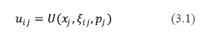
Where the vectors xj and pj represent the observed product characteristics and the price of the product, respectively. On the other hand ξij, captures the distribution of consumer preferences about the mean related to consumer i for product j. The specification of the utility function of consumer i for product j is then written as follows:
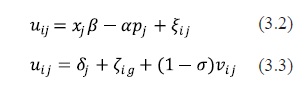
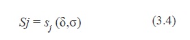
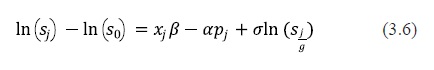
Where δj=xjβ-αpj is called the mean utility level of product j . I will assume that vijis an identically and independently distributed extreme value. Notice that αis interpreted as the disutility derived from prices and this parameter does not change across consumers. Moreover, ζg is common to all products in group g, given a consumer i. Finally, I should mention that the parameter σє[0,1] which is considered as a measure of the degree of correlation between alternatives belonging to the same group.
I have incorporated a nested logit framework for the consumer tastes because ξij=ζig+(l-σ) vij. is also an extreme value random variable since vij has the same distribution. Under this specification an individual will choose product j if the utility to enjoy this product exceeds the utility to be gained when product k was selected. That is, the choice is established when u ij≥uikfor j≠k.
In what follows, I will keep the same structure introduced by Berry (1994) in which the nested logit model was specified in terms of the market share functions. In that study, the market shares are transformed in such manner that those shares depend only on the mean utility level and the correlation coefficient:
Since I have assumed an extreme value distribution, the market shares of product j in group g is given by:
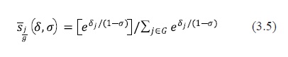
In order to present the analytical result, I should emphasize that the mean utility level of the outside good is set equal to zero i.e.,δ0= 0, . When there is an absence of the outside good, the consumers must choose from the inside goods and thus the demand will be determined only by the differences in prices. Therefore, the analytic expression is given by
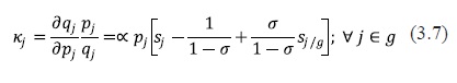
Where the market shares are defined by the following expressions sj= qj/ M, sj/g = qj/M gfor j = 0,1, ...,J. On the other hand, M, Mg and qj represent the size of the market, the size of the market segment and the quantity of product j on the market, respectively. Once the consumer's part has been set up, the own price elasticities can take the following form:
4. FIRM'S PROBLEM: PRICING EQUATIONS
This section will also be based on the work done by Berry (1994). I have assumed in this section a set of single product firms each producing a differentiated product. I have also assumed that the cost function is given by the following specification
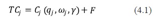
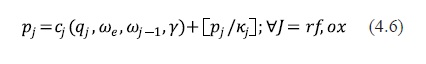
Where ωjis the input factor price related to product qj F is a fixed cost, and γrepresents the parameters associated to the input and quantity variables in the cost function. The marginal cost will be denoted as cj(qj,ωjγ) or comitting the arguments without loss of generality. In what follows, I will define the firm's problem and obtain the first order necessary conditions in order to specify the price-margin equations for a single product monopolistic competition scheme:
The list of prices and quantities {p1*,p2 *,...,pJ*;q1*,q2*,...,qj* } is a Bertrand-Nash equilibrium if:
i) Given p1*,... pj*-1, pJ*+1,..., pj*; Pj solves the following problem:
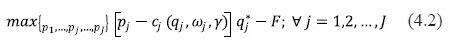
ii) qj*=Msj* (δ,Ï);p1*,p2*,â¦,pJ*;q1*,q2*,â¦,qJ* ⥠0.
Observe from equation (4.2) that a Bertrand market structure has been assumed implying that the firms set prices rather than quantities. Bertrand structure is more convenient given the fact that firms are able to modify prices faster and at less cost than to change quantities due to the technological and capacity constraints related to them. The first order necessary conditions of the above problem are as follows:
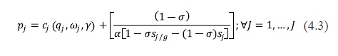
Where equation (4.3) implies that the price of product j=1,2,...,J is equal to the marginal cost of product j plus a markup expression. Notice that the latter term is a function of the correlation coefficient, the marginal utility of income, and the market shares. If σ=0, in this case, the product shares, Sj, only affect the markup and conversely if σ=1,sj/g is the only important factor in the markup.
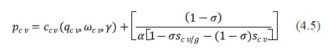
One of the main contributions of this study is the calculation of the gasoline price effects when the ethanol subsidies are eliminated. Recall that I have clasiffied the gasoline market products into three categories. Two of them are blended with ethanol such as the reformulated and the oxygenated gasolines while the conventional gasoline is not blended with any type of oxygenates. Equation (4.3) can be written in order to be product specific as follows:
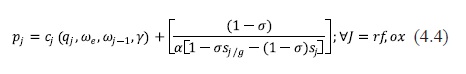
Where ωeωj-1 represents the ethanol price and other input prices utilized in the production process to obtain the reformulated and oxygenated gasolines. Equation for the conventional gasoline is given by:
The second term of equation (4.4) can be expressed as pj./ Kj and therefore:
If the cost function is twice continuously differentiable, then C* satisfies:
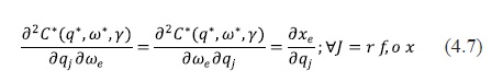
Where the last equality holds by introducing the Shephard's Lemma and thus Xe represents the input demand for ethanol. I then take the derivative of equation (4.6) with respect to subsidy, s, and thus:
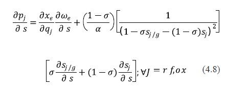
Since the own price elasticity, kj. , is a function of the σ,s.j/g and Sj, the intuition provided by equation (4.8) could be analyzed in three cases which are described below. As I have mentioned previously σis defined as the degree of intragroup correlation. In other words, as σ→0 the within group correlation of utility goes to one and as σ→0 the correlation between products belonging to the same group goes to zero. Recall that this relationship is established in terms of product characteristics. Therefore, if consumers think that two products in the same group have the same characteristics, these products will be highly correlated, and thus, this could be thought of as if consumers are not able to distinguish the difference between a product environmentally improved such as either the reformulated or oxygenated gasoline and non-quality improved product such as the conventional gasoline.
Case I: If σ→1, sj/g> 0 and sj> 0, then kj → -∞. Therefore, the price effects related to the blended products are given by:
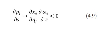
When the blended product demand curves are perfectly elastic, the variation of the blends prices with regard to subsidy changes will depend on ∂X e / q j . and ∂X e / σ j which are positive and negative respectively. The first term implies that an increase in the production of either the reformulated or the oxygenated gasoline will produce a positive impact on the demand for ethanol. On the other hand, the second term of equation (4.9) establishes a negative relationship between the subsidy and the ethanol price. Therefore, this theoretical framework suggests that the subsidy will be negatively related to the blends prices, in other words, a decrease in the ethanol subsidies will produce an increase in the prices associated with the blended products.
Case II: If σ→0,sj/g> 0 and sj>0, then kj →αpj (sj-1 ). then. Therefore, the price effects are given by:
In this case, the price effects will depend on the market shares of the products blended with ethanol at the nationwide.
Case III: If σє(0,1), sj/g > 0 and sj. > 0, then the price effects are determined by equation (4.8). Equations (4.8) and (4.10) would suggest a negative relationship between prices and subsidies if the first part of the equation, which is negative, dominates the second term.
On the other hand, I take the derivative of equation (4.5) with respect to subsidies in order to obtain the effect on conventional gasoline prices under the hypothetical scenario. I get the following expression:
Equation (4.11) might reflect a negative relation between conventional gasoline price and subsidies since the derivatives of the market shares with respect to subsidies are also negative. A decrease in the ethanol subsidies might produce a reduction of the market shares associated with the blended products and therefore this might imply an increase in either the conventional gasoline market share or the outside alternative providing the intuition related to the sign of these derivatives. Similarly, equation (4.11) could be analyzed into three cases:
Case I: If σ→1, scv/g , > 0 and scv > 0, then kcv →- oo and then. Therefore, the magnitude of the price effects related to the conventional gasoline tends to be negligible because the demand for this gasoline is perfectly elastic. For instance, a decrease in the ethanol subsidies will produce a reduction of the blended products market shares, and therefore, the fuel market will experience an increase in the market share associated with the conventional gasoline. Consequently, the increase of the conventional gasoline market share might pressure its prices to be higher, but since the demand for this type of gasoline tends to be perfectly elastic, in this case, the magnitude of the price effects might be negligibly small.
Case II: If σ→0, scv/g > 0 and scv > 0, then kcv →α pcv (scv -1). Therefore, the price effects are given by:
In this case, the price effects will depend exclusively on the market shares of the conventional gasoline at the nationwide.
Case III: If σ ε (0,1), scv/g > 0 and, then the price effects are determined by equation (4.11) which indicates a negative relationship between conventional gasoline price and ethanol subsidies since σscv/g / σ s < 0 and σscv / σ s < 0.
5. DATA
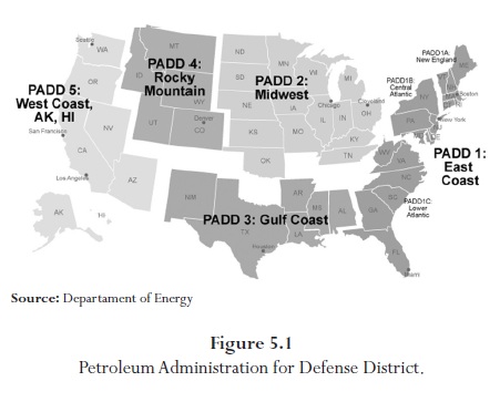
I have gathered information on the prices and sales of the different liquid fuel categories that were previously defined. Moreover, I have collected information on the weight and volume percentages of the distinct types of additives used in the production of gasoline programs such as the reformulated gasoline. The former data was collected from the Energy Information Administration (EIA) data base while the latter information was obtained from the reports elaborated by the Environmental Protection Agency (EPA). I worked with all this information by the Petroleum Administration for Defense Districts (PADDs), which are depicted in the figure (5.1), for 1995/2005 period.
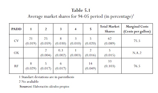
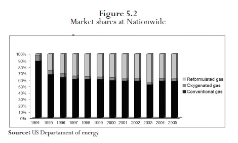
Table 5.1 presents some descriptive statistics about the data base utilized in this study. In 1994/2005 period, conventional gasoline accounts on average for 62% of the gasoline market while the oxygenated and reformulated gasoline are about 4.96% and a 33.04%, respectively. Table 5.1 also provides information on how the consumption related to these three products is split among the 5 regions in the country. In fact, two of the most important regions in terms of consumption of conventional gasoline are the East coast and the Midwest accounting for the 21 and 25 per cent on average while the West coast registers the most important participation with regard to the consumption of the reformulated gasoline.
The information obtained from the Department of Energy is in terms of thousands gallons a day by year and by districts. Figure (5.2) describes the evolution of the market shares related to these three types of gasoline considered in this study at the nationwide. It is worth noting that the market shares of the conventional gasoline has been declining since the introduction of the oxygenated and reformulated programs in 1994. The latter product has been gaining market share since then. The reformulated gasoline has been growing on average at the rate of 11.74% while the conventional gasoline has been decreasing at 4.48% on average in this period.
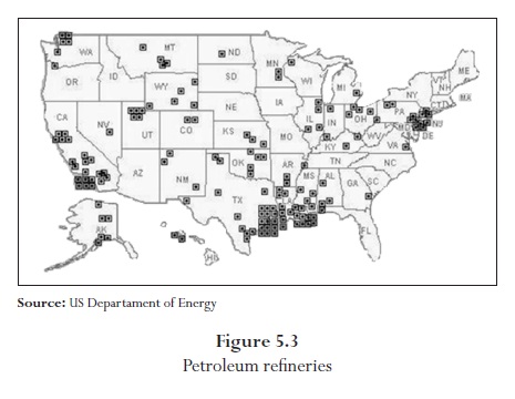
Figure (5.3) Depicts the concentration of the refineries across the country. Most of the refineries are located on the West and Gulf coasts, primarily because of access to major sea transportation and shipping routes.
On the other hand, I estimated a short-run multiproduct symmetric generalized Leontief cost function to approximate the refineries and blenders' technology. I assumed that this flexible functional form reflects the fact that refineries and blenders used some inputs: crude oil, natural gas and some oxygenates such as ethanol and MTBE, to produce aggregate outputs such as the reformulated gasoline, the conventional gasoline and others. I also included the fixed asset and energy inputs in our cost function specification. These variables represent our quasi-fixed inputs. Therefore, I have employed those estimated marginal costs as starting points to accomplish our simulation, otherwise the model would not have been calibrated precisely.
Finally, the Reformulated Gasoline (RFG) Surveys Oxygenate Information served to calculate the demand for different oxygenates whose methodology is explained later on in this work. Table 5.2 contains the average oxygenate concentration in terms of volume percent by districts for the period under analysis. Note that this information reflects the impacts of the ban related to the MTBE on the demand for oxygenates. A year later the ban of MTBE entered in effect, the demand for ethanol rose substantially while the MTBE experienced a consistent reduction at the nationwide.
6. METHODS AND PROCEDURES
The main justification for the application of this methodology is the lack of the household's information that would have served to estimate the equilibrium parameters and conditions. However, this method could become a very appealing procedure that policy makers could utilize in order to capture the economic effect to suppress the subsidies in the U.S. biofuel market.
This methodology is based on the study done by Ivaldi and Vibes (2005). The authors created this algorithm to simulate many scenarios in the German passenger rail and air transport industries. They simulated some potential scenarios such as the entry of a Low Cost Airline (LCAs), the entry of a low cost train and the presence of a new kerosene tax in this market. The deregulation in these industries along with the development of high speed technology that has reduced the gap between air and train travel time and the presence of low cost airlines which offer affordable tickets to an important market share of the population have boosted the competition between rail and air transportation. Therefore, passengers can decide between several modes and even several companies or alternatives between modes to obtain the transport service. These authors present a simulation model to analyze not only the inter modal competition, but also the competition within the same type of transportation. Regulatory changes on a particular framework incorporating the problems originated from the lack of disaggregated information.
The simulation of the hypothetical situation associated with the entry of Low Cost Airlines resulted in decreases of the market shares of rail, car, incumbent airline and the outside alternatives; but the LCAs market share increased. Prices related to all modes of transportation experienced reductions with a biggest impact on the LCAs price. The authors obtained the same pattern under the different assumptions of the outside alternative market shares established in 20%, 35% and 65%. On the other hand, the entry of a Low Cost Train (LCT) corresponds to a structural change in the market with very important consequences in the leisure segment. Prices declined for all alternatives, and the prices of the leisure segment of this transport mode declined by more than 20%. All transport mode market shares dropped favoring the participation of the new entrant, but it is worth mentioning that the business segment was less responsive since consumers in this segment do not appreciate land transport. The incumbent train company was not displaced by the new entrant due to the presence of imprecise information on the price differential and some other external considerations for the consumers. Finally, the authors evaluated the effect of a new kerosene tax manifested in an increase in airlines costs. The introduction of this new tax increased airline prices about 10% and all the other transportation modes experienced increases in smaller magnitudes. The increases in the tariffs produced that airlines released some traffic which was partly absorbed for other modes and even for the outside alternative.
This model has served to evaluate the effects of both structural and regulatory changes on a particular framework incorporating the problems originated from the lack of disaggregated information.
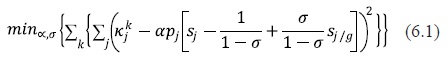
For the calibration of this model, I will need to compute demand elasticities, marginal costs and demand parameters as well. The equilibrium solutions are obtained by using the system of equations (3.6), (3.7) and (4.4). This model is solved in several steps: i) First, the demand parameters and are calculated by using the equation (3.7). I generate a random vector of elasticities establishing coherent assumptions on their distributions. In order to make consistent assumptions with regard to the vector of elasticities, I have used the estimated elasticities and their standard deviations recovered in the survey done by Dahl and Sterner (1991). This paper is a collection of studies on the U.S. gasoline demand elasticities. This survey classified the studies by data type and by different categories of model, the authors found a fair degree of agreement with regard to average short-run and long-run income and price elasticities7. The vector of elasticities is assumed to be normally distributed with one thousand repetitions. The demand parameters and are found by minimizing the average difference between the random vectors of elasticities and their associated expression proposed by Ivaldi and Vibes:
2) Second, I compute the marginal costs using the system of equations (4.3). I repeat this procedure until the vector of di-ferences between the computed and observed marginal costs were negligibly small. By following these steps, I was able to save the latest values for α, σ marginal costs and the vector of own prices elasticities by districts.
Finally, the market share of the outside good8 has been assumed to take the values of 3% and 5%. In other words, the percentage of consumers who do not consume gasoline could amount for those values restricting the gasoline market size assumption.
7. SIMULATION RESULTS ON THE U.S. FUEL MARKET
This simulation consists in capturing the economic effects of eliminating the subsidies associated to the biofuel production in 1995-2005 period. Ethanol production has been motivated among other incentives for the subsidies. Therefore, it would be interesting to question to what extent this biofuel has been able to compete on its own merits. Certainly, an absence of ethanol subsidies will have an impact on the marginal costs associated to the blended products such as the oxygenated and reformulated gasoline. I have calculated that an average increase of 10% in the marginal costs of these products have been translated in three effects: i) a decrease in the market shares associated with the ethanol-gasoline products, ii) price increases of ethanol blended products, and iii) a reduction of the demand for oxygenates due to the decrease of reformulated gasoline market shares.
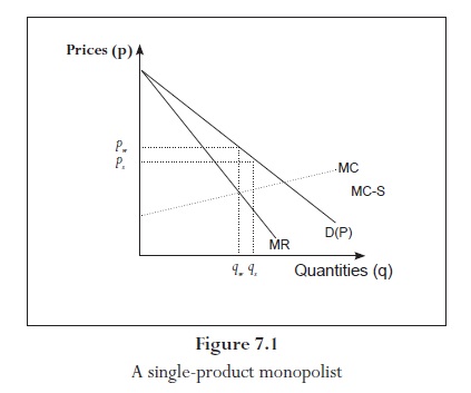
The following results coincide with the intuition provided by the economic theory on single-product monopolist competition. As I can observe in the figure (7.1), when I assume that the subsidies, S, are suppressed, the marginal cost curve will shift up and therefore a new equilibrium is reached.
This new equilibrium is denoted by pw and qw terms that represent the prices and quantities without subsidies. It should be noted that the new equilibrium establishes an increase in prices and a decrease in quantities under the situation in which the blender's credits are eliminated.
Recall that there are two blended products, reformulated gasoline and oxy-fuels, which are currently enjoying the subsidy benefits and thus, these products will experience decreases of their market shares under the hypothetical situation.
Notice that the diminution of the reformulated gasoline's market share implies a decline of the required amount of oxygenates used in the blending processes.
The simulated results confirmed this economic intuition and are reported in the following tables.
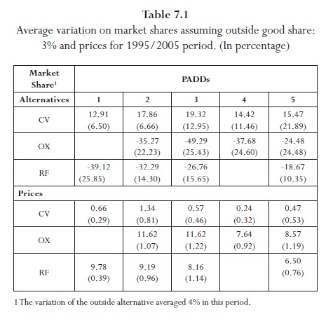
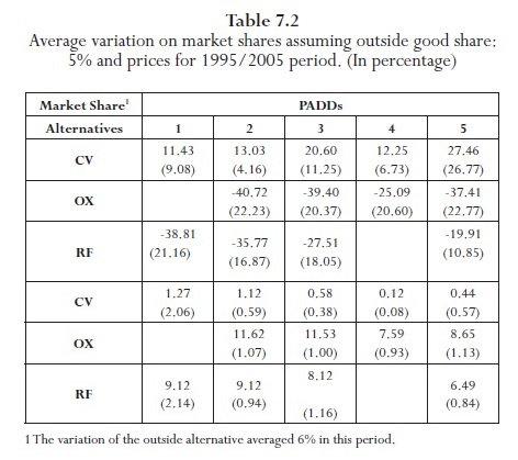
Tables 7.1 and 7.2 contain information on the percentage changes of market shares and prices under the hypothetical scenario where the blender's credits are phased out for 1995/2005 period. I assume that the outside good's market share is either 3% or 5%. Notice that the elimination of ethanol production subsidies, manifested as an increase in marginal costs, have decreased the market shares of both the reformulated and oxygenated gasoline on average. These decreases are in a range between 18.67 and 49.29 per cent. Conversely, the conventional gasoline market shares have experienced increments in all the regions. With absence of subsidies, consumers were not only willing to switch their consumption decision from the ethanol blends to the regular gasoline across petroleum districts, but they would also have been willing to take public transportation, bike or walk more frequently. The latter conjecture is sustained by the average increase associated to the outside alternative market share which is about 4% and 6% respectively.
It is worth mentioning that one of the relevant contributions of this paper has been the approximation of the gasoline price variations related to the relaxation of subsidies in the U.S. biofuel industry. Notice that all the PADDs have experienced price increases. These increases are also in terms of average for 1995-2005 period. As I observe from those tables, conventional gasoline has captured some impact on its prices which are in a range between 0.12 and 1.34 per cent. On the other hand, among the ethanol blends, the oxygenated gasoline has experienced a greater increase than that observed in the reformulated gasoline prices for the period of analysis.
8. SIMULATION RESULTS ON THE U.S. OXYGENATE MARKET
In order to calculate the demand for oxygenates under the hypothetical situation in which the ethanol's subsidies are relaxed, I have assumed that there is only two oxygenate types in the U.S. market such as ethanol and MTBE. Either of these two oxygenates could be used to produce the reformulated gasoline. I have also assumed that the blenders are associated with Constant Elasticity of Substitution (CES) production function9. The CES production function takes the following form:
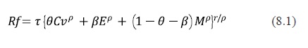
Where Cv, E, and M represents the amounts of conventional gasoline, ethanol and metryl tertiary butyl ether(MTBE) utilized to produce the reformulated gasoline, RF. The degree of homogeneity of the function has been denoted by r,t 0 represent the efficiency parameter wich is commonly associated with the size of the production function. Morover, θ Βε [0,1] denote relative factor shares and finally p represents the substitution parameter used to derive the elasticity of substitution.
Therefore, the blender's problem consist on finding the list of inputs [Cv*, E*,M* }, given the list of prices [Pcv*,PE*,PM* }; such that [Cv, E, M}solve the following maximization problem:
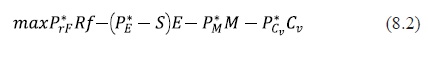
Subject to equation (8.1) and the non-negativity constraint. Assuming interior solutions and replacing the production function in the equation (8.2), the first order necessary conditions of the above problem are as follows:
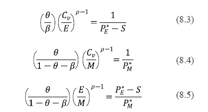
It is worth noticing that the assumptions of constant returns to scale, i.e. r = 1, the normalization of the conventional gasoline price and the presence of ethanol subsidies, S, have been introduced in the maximization problem. Re-arranging the above system of equations, I found the following expressions:
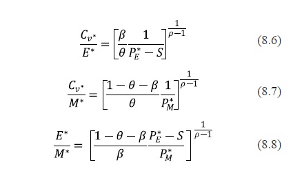
The main goal of this part of the analysis is to obtain the ratios under both scenarios, with and without ethanol's subsidies, in order to identify some substitution patterns between ethanol, MTBE and the conventional gasoline; but the parameter is unknown. Therefore, I simulated the above system of equations by creating a grid of values for rho. This simulation was possible since I have information on prices and on the oxygen requirements imposed by the Environmental Protection Agency (EPA) in terms of weight percent described in Table 5.2.
The simulation proceeded by executing the following steps: i) p was assumed to be either uniformly or normally distributed, ii) the random numbers of p served to generated the different input ratios taking into account the hypothetical situations, iii) the computed input ratios were compared with the actual data, and iv) this loop ended when the difference calculated in iii) was negligible obtaining the most appealing value for the parameter p under this criterion. The maximum level of tolerance for the difference between input ratios was established in twenty percent. The results are depicted in the following graphics:
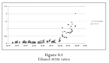
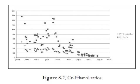
Figure (8.1) indicates that the elimination of the ethanol's subsidies would have induced the blenders to substitute ethanol for another oxygenate type, in this case MTBE, to satisfy the EPA regulations. The darker points represent the situation in which the subsidies have been suppressed and those points are related to lower ethanol-MTBE ratios compared with the scenario in which subsidies are included. As a result of this substitution pattern between ethanol and MTBE, the conventional gasoline-ethanol ratio increases under the elimination of the ethanol's subsidies. The latest is illustrated in Figure (8.2). Obviously, the higher the elasticity of substitution, the lower the ethanol-MTBE ratios, this is described in Figure (8.3).
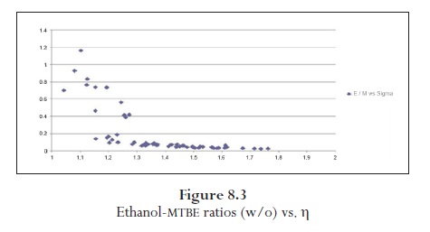
According to these simulation results, the suppression of the ethanol's subsidies would have reduced the ethanol-MTBE ratio in 55:14% on average with a standard deviation of 0.123, while the elasticity of substitution averaged 1.38 with a standard deviation of 0.1766. The details of these results are reported in the Appendix.
CONCLUSIONS
The Ivaldi-Vibes algorithm has proven to give very appealing results in its economic applications. I believe that this algorithm has also provided reasonable results with regard to the simulation associated with a hypothetical elimination on ethanol production subsidies. I have reported that, under this hypothetical scenario, the individuals were not only willing to switch their consumption decision, but they were also willing to consider alternative modes of transportation such as the public transportation, bike or walk. In other words, the outside alternative market share increased about 4% and 6%; and the conventional gasoline market shares increased as well, while the others related to the ethanol blends experienced decreases across all petroleum districts. I have also simulated the impact on the gasoline prices. At the best of my knowledge, there is no a study which has tried to capture the impact on the gasoline price under the elimination of the ethanol subsidies. It should be noticed that the conventional gasoline prices have increased in a range between 0.12 and 1.34 percent.
I could conclude many lessons from this study: i) this algorithm allowed the simulation of the market shares for the distinct types of gasoline under the hypothetical scenario. The oxygenated gasolines experienced decreases in their market shares and therefore those looses were manifested in increases of the conventional gasoline and the outside alternative market shares, ii) As results of looses in the market shares and increases in prices of the oxygenated gasolines, firms producing conventional gasoline could gain more profit by exercising its monopoly power and establishing higher prices in the range mentioned before. Therefore, this methodology could be considered a complementary tool for the competition analysis in this industry, iii) since there is no households data that allows the application of more precise econometric methods, this framework permits to model some features of the gasoline market and to analyze some changes in the tax-subsidy scheme.
This algorithm could be extended to introduce the analysis of other industry policies such as the Renewable Fuel Standards and to measure its impacts on the gasoline and oxygenate markets.
On the other hand, as it is well known, different types of oxygenates are blended with the regular gasoline satisfying the EPA regulations. Therefore, the reduction in the reformulated gasoline market shares implied a trade off in the demand for these oxygenates whose variation rates were reported in Table A.6. It should be pointed out that the elimination of ethanol's subsidies has shown a substitution pattern between ethanol and MTBE. Under this scenario blenders are induced to replace the most expensive ethanol alternative for another type of oxygenate, in this case MTBE. Evidently, the ethanol-MTBE ratio decreased and this reduction averaged 55:14% with a standard deviation of 0.123. The measure of goodness of fit associated to this simulation model is about 48.78%.
This method could serve as a basic tool for both firms and regulators viewpoints. Even though, I certainly believe that many assumptions could be relaxed. One of the assumptions that has been eliminated in this paper is related to the marginal costs. The marginal cost was not assumed to be constant; in fact, these marginal costs were calculated in the first chapter of this dissertation by using a flexible functional form cost function. On the other hand, possible extensions that I might intend to address are the hypothetical situation in which a finite number of potential plants decide to enter in the gasoline production market and the introduction of the Renewable Fuel Standard objectives. Finally, other extensions could be associated to the assumptions of market structure competition and prices.
Pie de paginas
1 Equivalently, this excise tax represented 0.40 US$/gallon of pure ethanol.
2This loans had a limit over 1 million dollars.
3 The demand for ethanol is determined by its two end uses which are as conventional gasoline volume extender and as oxygenate.
4 Reformulated gasoline must contain a minimum of 2.0% of oxygen. Because of the ban on the use of MTBE, Ethanol might become the most common source to satisfy the oxygenate requirement imposed on the gasoli ne production. Notice that 10% ethanol blends contain about 3.5% oxygen in the fuel. Therefore, the oxygen content requirement can be accomplished using a 7.7% blend of ethanol with conventional gasoline.
5 VOC stands for volatile organic compounds.
6 The PADDs are divided into five categories. PADD I (East Coast): PADD IA (New England): Connecticut, Maine, Massachusetts, New Hampshire, Rhode Island, Vermont. PADD IB (Central Atlantic): Delaware, District of Columbia, Maryland, New Jersey, NewYork, Pennsylvania. PADD IC (Lower Atlantic): Florida, Georgia, North Carolina, South Carolina, Virginia, West Virginia. PADD II (Midwest): Illinois, Indiana, Iowa, Kansas, Kentucky, Michigan, Minnesota, Missouri, Nebraska, North Dakota, Ohio, Oklahoma, South Dakota,Tennessee,Wisconsin. PADD III (Gulf Coast):Alabama, Arkansas, Louisiana, Mississippi, New Mexico, Texas. PADD IV (Rocky Mountain): Colorado, Idaho, Montana, Utah, Wyoming. PADD V (West Coast): Alaska (North Slope and Other Mainland), Arizona, California, Hawaii, Nevada, Oregon,Washington.
7 Dahl and Sterner (1991) did not consider estimation on seasonal data and some inappropriate model formulations.
8 According to the Bureau of Transportation through the OmniStats in 2003 reported that 95% of individuals on one typical day last month either drive or ride in a personal vehicle, company car, carpool, vanpool while the remainder took public transportation, biked or walked to get to work.
9 The CES production functions were introduced by Arrow, Chenery, Minhas and Solow (1961).
References
Berg, C. (2004). World Ethanol. An analysis of global competitiveness. World Ethanol and Biofuels Report, 5. [ Links ]
Berry, S. (1994). Estimating discrete-choice models of product differentiation. The RAND Journal of Economics, 25 (2) 242-262. [ Links ]
Dahl, C. & Sterner, T. (1990). Analyzing gasoline demand elasticities: A survey. Department of Economics, Louisiana State University. [ Links ]
Dipardo, J. (2005). Outlook for biomass ethanol production and demand. Energy Information Administration. [ Links ]
Dixit, A. & Stiglitz, J. (1977). Monopolistic competition and optimum product diversity. American Economic Review, 67, 297-308. [ Links ]
Duffield, J., Shapouri, H.,Graboski, M., McCormick, R. & Wilson, R. (1998). U.S. biodiesel development: New markets for conventional and genetically modified agricultural fats and oils. ERS Report 770. U.S. Department of Agricultural, Economic Research Service, Washington, D.C. [ Links ]
Eidman, V. (2006). Renewable liquid fuels: Current situation and prospects. Choices, 21 (1), 15-19. [ Links ]
Elobeid, A. & Tokgoz, S. (2006). Removal of U.S. ethanol domestic and trade distortions: Impact on U.S. and Brazilian ethanol markets. Center for Agricultural and Rural Development, Iowa State University. [ Links ]
Ivaldi, M. & Vibes, C. (2005). Intermodal and intramodal competition in passenger rail transport. University of Toulouse. [ Links ]
Kane, S. & Reilly J. (1989). Economics of ethanol production in the United States. U.S. Agricultural Economic Report, 607. Department of Agricultural, Economic Research Service, Washington, D.C. [ Links ]
[11] Koplow, D. (2006). Biofuels-at what cost? Government support for ethanol and biodiesel in the United States. Geneva, Switzerland: Global Subsidies Initiative of the International Institute for Sustainable Development. [ Links ]
Lindderdale, T. (1999). Environmental regulations and changes in the petroleum refinery operations. Washington, D.C.: Energy Information Administration. [ Links ]
Quear, J. & Tyner, W (2006). Development of variable ethanol subsidy and comparison with the fixed subsidy. West Lafayette, Indiana: Agricultural Economics Department, Pardue University. [ Links ]
Shapouri, H., Salassi, M. & Fairbanks, N. (2006). The economic feasibility of ethanol production from sugar in the United States. Washington, D.C.: Department of Agricultural, Economic Research Service, [ Links ]
Taheripour, F. & Tyner, W (2007). Ethanol subsidies, who gets the benefits? West Lafayette, Indiana: Department of Agricultural Economics, Purdue University. [ Links ]
Tirole, J. (1988). The theory of industrial organization. Cambridge, MA: The MIT Press. [ Links ]
