


 Inglês (pdf)
 Artigo em XML
 Referências do artigo
 Enviar este artigo por email
 Citado por SciELO
  Citado por Google
  Similares em
SciELO
Similares em
SciELO  Similares em Google
 Permalink
1 Introduction
Seasonal diseases in humans are inherent in the organic growth of man from infancy to old age. Some examples of such diseases are measles, diphtheria, chickenpox, cholera, rotavirus, respiratory syncytial virus (RSV ), vector-borne diseases including malaria and even sexually transmitted gonorrhoea 1. In the modeling of the transmission of seasonal diseases, several nonlinear models of ordinary differential equations have been used 2),(3. In these models, the variables commonly represent subpopulations of susceptibles (S), infected (I), recovered (R), latent (E), transmitted disease vectors, and so forth. Generally, the most important term is the nonlinear term βSI which comes from the law of mass action and where β is the transmission parameter of the disease 2. In these models, periodic continuous functions β(t) (called sometimes seasonally-forced functions) incorporate the seasonality of the spread of the disease in the environment 4),(5),(6),(7. As an example of a seasonally-forced function, many authors use the expression β(t) = b 0(1 + b 1 cos(2π(t + ϕ))), where b 0 > 0 is the baseline transmission parameter, 0 < b 1 ≤ 1 measures the amplitude of the seasonal variation in transmission, and 0 ≤ ϕ ≤ 1 is the normalized phase angle. Other examples of seasonal functions can be found in 5),(8),(6, where the models have a time dependent transmission rate. Recently, in 9),(10),(11),(12 deterministic epidemiological models have been studied, where the contact rate depends on more complex variables and flow parameters of one subpopulation to another depend on time. However, these models do not take into account the inherent randomness associated with the time variation of the data. Moreover, environmental fluctuations are some of the most important effects in real world systems. A large portion of natural phenomena does not follow a deterministic law exactly, but rather oscillates randomly around some average value 13.
In the seasonal epidemic models there are two environmental fluctuations that can be considered: the first is the natural and well recognized fluctuation of the seasonal transmission rate which is modeled by the seasonally-forced function β(t) and the second is the smaller random perturbations affecting the seasonal transmission rate which are modeled by Gaussian white noise. These last fluctuations arise from uncertainties and variations in environmental, demographic and all other parameters involved in the model system 14),(15),(16.
Thus, in this paper we propose to examine the effects of the stochastic process solution of the mathematical model presented in 17. The stochasticity or noise is introduced on the baseline transmission parameter of the model given in 17, with the parameter perturbation technique, which is a standard technique in stochastic population modeling 14),(18),(19. In addition it should be mentioned that several stochastic models have been applied to several issues including epidemics, for instance 20),(21),(13),(22),(23),(24. Other types of stochastic models, such Markov’s chain and graphs can be applied for several diseases with different characteristics 25.
Previous studies regarding positivity and boundedness of solutions of stochastic differential equation models have been developed without seasonal transmission parameters. In this paper we are interested in the introduction of stochasticity in the seasonal parameter in order to provide some additional degree of realism when compared with their deterministic counterparts 21),(26. The main reason to introduce environmental stochasticity is that this can be a driving force that may change the deterministic dynamics of models 5),(27. In addition, the positivity and boundedness of solutions are important to other nonlinear models that arise in sciences and engineering where uncertainty is included 28. Thus a very important issue that arises when stochasticity is introduced in the seasonal epidemic model is positivity and boundedness of the solution.
For stochastic modeling different types of perturbations or randomness can be included in the model 25),(28. However, in the art of modeling it is necessary to investigate which type of perturbation is more suitable for the particular disease. This issue is not a straightforward task and needs to be tackled with different statistical tools. However, each disease may have a different environmental stochasticity depending on the region. Historically, stochasticity has been introduced in many models of stock prices, economics, queueing theory, engineering, and biology. Nevertheless we do not rely on only this fact. For example, based on real hospitalization data of the respiratory syncytial virus (RSV ), we believe that the transmission of this type of disease is affected by several physical and social variables 29),(30. In fact RSV is an illness for which the timing and severity of outbreaks in a community vary from year to year 6),(31),(29. Here we assume that the transmission rate parameter of the RSV can be assumed equal to an average value plus a small time fluctuating term and this term follows a normal distribution with mean zero 32. Many parameters have variations of this type. Possible explanations of this fact are a noisy environment due to several factors, such as temperature, humidity, pollution, transport, population and others. Our approach is to perturb the transmission rate parameter of the RSV by a Wiener process. Thus, from a theoretical point of view we can rely on the existing framework for ordinary differential equations dealing with Gaussian white noise perturbations 33. Additionally it is important to mention that other parameters of the model such as birth rate can be also perturbed stochastically but generally, in epidemic models, the most sensitive parameter is the transmission parameter of the disease 34),(32),(35. However, future work may include the study of positivity and boundedness of solutions when all parameters are perturbed jointly.
This paper is organized as follows. Section 2 introduces a stochastic model for transmission of seasonal epidemic diseases in a population, where some stochasticity is introduced on the baseline transmission rate. In Section 3 we show the positivity of the solutions of the proposed stochastic model. Section 4 is devoted to the analysis of the existence and dynamical behavior of the solutions in the disease free state. The the property of stochastically ultimate boundedness is proved in Section 5. In Section 6, numerical simulations using some parameter values from clinical data of hospitalized individuals due to the respiratory syncytial virus RSV of the Spanish region of Valencia are presented in order to support our previous analytical results. Finally, in Section 7 discussion and conclusions are presented.
2 Derivation of the stochastic model
In (17) a generalized epidemic SIRS seasonal model dealing with population proportions of susceptibles S(t), infected I(t) and recovered R(t) has been presented and the authors showed the existence of periodic solutions, where the contact rate is a continuous periodic function β(t). The system is a first order ordinary differential equation of the form
 ()1
()1
where:
1. The population is divided into three classes:
Proportion of susceptibles S(t), who are all individuals that have not the virus,
Proportion of infected I(t), being all the infected individuals having the virus and able to transmit the illness,
Proportion of recovered R(t), who are all the individuals not having the virus and with a temporary immunity.
2. The instantaneous birth rate µ(t) > 0 for all t ≥ 0, and equal to the instantaneous death rate, and we take it to be a continuous function.
3. For all the classes it is assumed the birth rate µ(t) is the same, because we assume that deaths associated with the disease are small.
4. The contact transmission rate (called seasonally-forced function) is a function β(t) between classes S(t) and I(t), and is a continuous periodic function, which satisfies
It is very common to approximate  , where b0 > 0 is the baseline transmission parameter, 0 < b1 ≤ 1 measures the amplitude of the seasonal variation in transmission and 0 ≤
  ≤ 2π is the normalized phase angle (6).
The instantaneous per capita rate of leaving the infective class I(t) is called ν(t) and the instantaneous per capita rate of recovered class R(t) is called γ(t), which are non-negative, continuous and bounded functions in [0, ∞[.
It is assumed that γ(t) < ν(t), for all t ≥ 0, i. e., the per capita rate of recovery is smaller than the per capita rate of leaving the infective and also that µu, νu, γu , and µl, νl, γl are positive real numbers defined
by

It should be mentioned that generally the recovery parameter ν(t) and the loss of immunity parameter γ(t) are assumed constant but here we include a more general case where these parameters can vary with time. On the other hand, birth and death rate µ(t) are assumed varying with time in other epidemic models where the size of the population is varying with time 2.
Fluctuations in the environmental conditions are some of the most important factors affecting real world systems. A large part of natural phenomena do not follow deterministic laws exactly, but rather oscillate randomly around some average value (13). Therefore, in this paper we propose to examine the effects of the introduction of environmental noise on the positivity and boundedness of the stochastic process solution of the mathematical model proposed in 17. The stochasticity or noise is introduced by perturbing the baseline transmission parameter b 0 in the model. This is a common technique used in stochastic population modeling 14),(18),(19),(36),(37 and it allows us to get analytical results 38),(18),(19),(39),(36),(37.
Let us now consider the model (1) with the perturbation on the baseline transmission parameter b 0 given by white noise. The use of Gaussian white noise is a good hypothesis in this model since it is assumed that the baseline transmission parameter oscillates randomly around some average value, due to some time varying disturbances. It is important to remark that this is the usual way to consider fluctuation in stochastic population dynamics 13. In addition, the transmission parameter seems to be the parameter with faster variability since it depends on many variables such as temperature, humidity, pollution, transport and population that can vary every single day. On the other hand, the death and birth rates vary much more slowly and the recovery rate varies much less since is an intrinsic value of the disease.
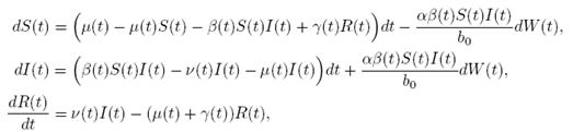
In this way, if a stochastic perturbation is made on the baseline transmission parameter b 0 as in 20),(21),(23, an Itoˆ type stochastic
differential system of the following form is obtained:
 ()2
()2
where X(t) = (S(t), I(t), R(t))
T
and the solution {X(t), t ∈ [t
0
, tf
]} is an Itoˆ process, f is the continuous deterministic component or drift coefficient, g is the continuous random component or diffusion coefficient33, defined by 
 . Thus, f is an d-vector valued function, g is an d×m matrix-valued function, and W (t) is a m-dimensional stochastic process having scalar Wiener process components. For our particular
case, m = 1 and d = 3. Here, the perturbation to the baseline transmission parameter b 0 is introduced in the following form
b˜0 = b 0 + αη(t),
where α ∈ R is the intensity of the noise and η(t) is defined as the formal derivative of a standard Wiener process (a formal derivative because W (t) has probability one of being nondifferentiable). Since the Gaussian white noise has mean zero and the intensity of noise is small in comparison to the baseline transmission parameter b
0, one gets positive values for b˜0 . Since negative values make no sense, the very few negative values that may be produced during the simulation will be discarded. The new transmission rate is given by: 
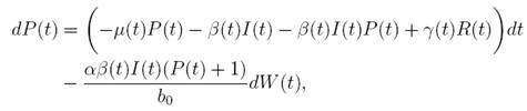
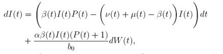
 . Thus introducing the perturbation on equation (1) and multiplying by dt, one gets the following stochastic differential system given by
 ()3
()3
with initial data 
3 Global positive solution
Since (3) represents a population system, it is important that we do not obtain negative values. Thus, we must first prove the positivity of the solutions. Unless otherwise specified, let  be a complete probability space with a filtration
  satisfying the usual conditions (i.e. it is increasing and right continuous while
  contains all P-null sets). Let W (t) be the one-dimensional Brownian motion defined on this probability space. Let X(t) = (x
1(t), x
2(t), x
3(t))
T
and
contains all P-null sets). Let W (t) be the one-dimensional Brownian motion defined on this probability space. Let X(t) = (x
1(t), x
2(t), x
3(t))
T
and
The following theorem guarantees the existence and uniqueness of the solution of system (3).
Theorem 3.1.
Assume that µu, νu, γu, b
0
, are positive real numbers. Let X(0) = (S(0), I(0), R(0))
T
∈ Ω be any initial condition. Then, there is a unique solution X(t) = (S(t), I(t), R(t))
T of the system (3) for t ≥ 0 and the solution will remain in
 with probability 1
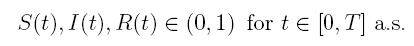
Proof. Let Z(t) = S(t) + I(t) + R(t). We can see from (3) that if X(0) = (S(0), I(0), R(0)) T ∈ Ω, and t ∈ [0, T ] almost surely (a.s), then

for t ∈ [0, T ] a.s. Therefore, we obtain that Z(t) < 1, i.e.,
 ()4
()4
It is clear that the coefficients of the system (3) are locally Lipschitz continuous. Thus, for any given initial value X(0) ∈ Ω there is a unique maximal local solution X(t) on t ∈ [0 , τe ] , where τe is the explosion time, see 40. In order to prove that the solution is global, it is necessary to show that τe = ∞ a.s. Take k 0 an integer, sufficiently large so that if X(0) ∈ Ω, then every component of X(0) lies within the interval [1/k 0 , 1). For each integer k ≥ k 0, we define the stopping times


with the agreement that inf ∅ = ∞ (where ∅ denotes the empty set). Clearly the sequence { τk } is increasing when k → ∞. Is clear that τ ∞ ≤ τe a.s. Thus, if we prove that τ ∞ = ∞ a.s, then τe = ∞ a.s, and X(t) ∈ Ω a.s, for all t ≥ 0. We prove now that τe = ∞ a.s.
Define the function V: (0, 1) × (0, 1) × (0, 1) →  given by
V (x 1 , x 2 , x 3) = − ln(x 1) − ln(x 2) − ln(x 3).
Using Itoˆ’s formula, for T > 0, t ∈ [0, T ∧ τk ] to X(t) = (S(t), I(t), R(t)), we obtain that
and using (3) we obtain
Thus, we get the following expression
Now, since S(t), I(t), R(t) ∈ (0, 1), for all t ∈ [0, T ∧ τk ] a.s., and with
 , one gets that
 ()5
()5

Therefore, integrating both sides of (5) from 0 to T ∧ tk , and after taking the expectation on both sides, one obtains that
 ()6
()6
Since V (X( τk ∧ T )) > 0. Then
 ()7
()7
≥ E[V (X( τk ))χ ( τ k ≤T )],
where
χB
is the characteristic function of B. Now, for
τk
, there is some component of X(
τk
), say S(
τk
), such that 0 < S(
τk
) ≤  < 1.Therefore, V (X(τk)) ≥ −
  . Thus,
 ()8
()8
From (6)-(8), it follows that
Letting k → ∞, for all T > 0, we obtain P(τ ∞ ≤ T ) = 0. Hence, P(τ ∞ = ∞) = 1. Thus, as τe ≥ τ ∞, then τe = τ ∞ = ∞ a.s. The proof is completed. ◆
Corollary 3.1. The set Ω is almost positively invariant by the system (3), that is, for X(0) = (S(0), I(0), R(0)) ∈ Ω, it holds that P[X(t) = (S(t), I(t), R(t)) ∈ Ω] = 1, for all t ≥ 0.◆
4 Local behavior
In this section we analyze the existence and dynamic behavior of the solutions in the disease free state.
4.1 Existence of the equilibrium disease states
The following theorem shows the existence of a disease-free equilibrium point.
Theorem 4.1. If βu < νl, then the system (3) is globally asymptotically stable, in the sense that for any initial value X 0 ∈ Ω, the solution X(t) will tend to the equilibrium point (1, 0, 0) asymptotically with probability 1.
Proof: We consider the second equation of system (3). Thus, for I(t), if I(0) > 0, we can use the function V 2(t) = ln(I(t)), with I(t) ∈ (0, 1). Applying Itoˆ’s formula, one obtains that
Then
Simplifying and dividing the above inequality by t > 0, it follows that
i.e. ,
 ()9
()9
Using the fact that lim  a.s. 23, one gets
 a.s, where θ =
βu
−
νl
−
µl
. Then one obtains that
a.s, where θ =
βu
−
νl
−
µl
. Then one obtains that
 ()10
()10
Since, I(t) > 0, for all t ≥ 0 a.s., we get  , a.s.
Now, from the third equation of system (3) it follows that
and from (10) we have that
 () 11
() 11
Therefore, if follows that  a.s. Finally, using Theorem (3.1) we can obtain that
  , a.s. Thus, the proof of the theorem is completed. ◆
4.1 Behavior around of disease free
The following theorem, shows that the solution of system (3), is oscillatory around of point (1, 0, 0), if βu < νl. Furthermore, the intensity of this oscillations depends of α.
Theorem 4.2. Under the hypothesis of Theorem 4.1, and if X0 ∈ Ω, then the solution X(t) of model (3), has the property

a.s.,
where, 
Proof. By making the change variable P (t) = S(t) − 1, in the system (3), this can be written as
 ()12
()12
 ()13
()13
 ()14
()14
Define a function, such that V
3(P, I, R) = (P + I)2 + c
1
I + c
2
R, with where P ∈  , I, R ∈ Ω, and c1, c2 are positive constants to be determined later. Is clear that V3 > 0, then
Thus, from Corollary 3.1, 0 < S(t), I(t), R(t) < 1 a.s, then P (t) < 0
a.s. Furthermore, from the hypothesis it follows that
Choosing c1 , c2 , such that  and −
c1
(
νl
+
µl
−
βu
) + c
2
νu
= 0, it follows that
and −
c1
(
νl
+
µl
−
βu
) + c
2
νu
= 0, it follows that
 (15)
(15)

Now, integrating both sides of (15) from 0 to t, and taking expectation, one gets that
Putting  , we obtain that
5 Global behavior
Theorem 3.1 and Corollary 3.1, show that the solution of the system (3) with a positive initial value in Ω, will remain positive in Ω. The properties of positivity and nonexplosion are essential for a population system. Once they have been established, is very important to discuss some other properties of the solution of system (3). From a biological point of view, due to the limitation of resources, the property of stochastically ultimate boundedness is more desirable than the nonexplosion property.
First, we show that the solution of system (3) is asymptotically bounded. Thus, we show first an important result, and then the stochastically ultimate boundedness follows directly.
Theorem 5.1. If θ ∈ [1, ∞), and there is a positive constant H0 that is independent of the initial value X(0) = (S(0), I(0), R(0)) ∈ Ω, then the solution X(t) = (S(t), I(t), R(t)) of (3) has the property
 (16)
(16)
Proof. From Corollary 3.1, the solutions will remain in Ω, for all t ≥ 0 with probability 1, a.s. We set V 4(X(t)) = Sθ (t) + Iθ (t) + Rθ (t), with θ ≥ 1. Using the Itoˆ’s formula one gets the following,
 (17)
(17)
Where  Let k
0
> 0 be sufficiently large, such that for every component of X(0) lying within in the interval [1/k
0
, 1). For each integer k ≥ k
0, define the stopping time by
Let k
0
> 0 be sufficiently large, such that for every component of X(0) lying within in the interval [1/k
0
, 1). For each integer k ≥ k
0, define the stopping time by
Clearly τk → ∞, almost surely as k → ∞. It follows from (17) that
Letting k −→ ∞, one gets that

Therefore,
Since,  then
then
Thus,
Therefore, we can obtain
 where
where  . Thus, the theorem has been proved.
Definition 5.2. System (3) is said to be stochastically ultimately bounded if for any ε ∈ (0, 1) there exists a positive constant H = H(ε), such that for any initial value (S(0), I(0), R(0)) ∈ Ω, the solution X(t) = (S(t), I(t), R(t)) of (3) has the property
 (18)
(18)
Theorem 5.3. Under Assumption (5.1), the system (3) is stochastically ultimately bounded.
Proof. By Theorem 5.1, for θ = 3/2, there is ∆ such that
Let ε > 0 be given, we can choose  . Therefore, by the application of the Chebyshev’s inequality one gets that
 . This implies the proof of theorem.
6 Numerical simulations
In this section, numerical simulations using some parameters values from clinical data of hospitalized individuals due to the respiratory syncytial virus RSV of the Spanish region of Valencia are presented in order to support our previous theoretical results. In addition, we illustrate the effects of introducing stochasticity by means of numerical simulations. At first the deterministic model of RSV is simulated and later the stochastic model. The introduction of stochasticity into the deterministic model helps to understand the differences between the deterministic model and the real data of RSV . Thus, the stochastic model can be seen as a more sophisticated model.
The virus RSV is the cause of acute respiratory infections in children younger than 2 years old, mainly bronchiolitis and pneumonia. RSV is spread from respiratory secretions through close contact with infected persons or contact with contaminated surfaces or objects. This virus has been known since 1957, but only recently has the adult pathology been established. It is also the cause of 18% of the hospitalizations due to pneumonia in adults older than 65 41. RSV is a seasonal epidemic with minor variations each year and coincides in time with other infections as influenza or rotavirus, producing a high number of hospitalizations and, consequently, a saturation of Public Health Systems 42),(43),(44),(45. RSV also causes repeated infections throughout life, usually associated with moderate-to-severe cold-like symptoms; however, severe lower respiratory tract disease can occur at any age, especially among the elderly or among those with compromised cardiac, pulmonary, or immune systems.
For the deterministic case model the parameter values have been taken from real clinical data of RSV hospitalizations of children younger than 4 years old during the period January 2001 to December 2004 from the CMBD (Basic Minimum Data Set) database of the Spanish region of Valencia 32),(44),(46. This data was collected weekly taking into account other diseases such as bronchiolitis and pneumonia. In addition some unknown parameters were estimated using the least-squares fitting procedure and using the hospitalization data. The mean square error obtained is less than 0.002. The graphical representation of the model fitting can be seen in Figure 1.
As can be seen graphically, the deterministic epidemic model (1) agrees well with the observed epidemic data, but it is important to notice that the hospitalization data is not exactly periodic as the deterministic model predicts 17. Thus, stochastic perturbations on parameters are a good explanation of these differences between the mathematical model and data, since without their use the simulation of the model will be exactly periodic. More details that include practical issues of the RSV mathematical modeling such as confidence intervals, parameter estimation, and numerical methods can be seen in 32),(42.
Figure 2: Numerical simulation of 6 trajectories of the stochastic model (3) computed using the Milstein scheme with perturbations on b0 in a range of 1%. The parameter values are b 0 = 37, b 1 = 0.31, ϕ = 0.9, γ = 1.8, ν = 36, µ = 0.009. The mean trajectory (dotted) is also included.
In the numerical simulation of the stochastic model it can be observed in Figure 2 that 6 different pathwise patterns occur with the mean trajectory included. Perturbations on b 0 in a range of 1% are used and Milstein numerical scheme 33 are applied to obtain the solutions of the stochastic system (3). All these trajectory solutions satisfy positivity and boundedness as the theoretical results predict.
Figure 3 Numerical simulation of 10 trajectories of the RSV stochastic model (3) computed using the Milstein scheme with perturbations on b0 in a range of 3%. The parameter values are b 0 = 37, b 1 = 0.31, ϕ = 0.9, γ = 1.8, ν = 36, µ = 0.009.
In order to give more support to our theoretical results, an extreme case with perturbations on b 0 in a range of 3% are used. As can be seen in Figure 3, the 10 pathwise trajectories with the mean trajectory are bounded and positive despite the use of large perturbations. It is important to remark that other perturbations in larger ranges have been taken and the positivity and boundedness are maintained.
Figure 4: Numerical simulation of 10 trajectories of the infectious from the RSV stochastic model (3) computed using the Milstein scheme with perturbations on b0 in a range of 1%. The parameter values are b 0 = 24, b 1 = 0.31, ϕ = 0.9, γ = 1.8, ν = 36, µ = 0.009.
Figure 5: Numerical simulation of 10 trajectories of the susceptible individuals from the RSV stochastic model (3) computed using the Milstein scheme with perturbations on b0 in a range of 1%. The parameter values are b 0 = 24, b 1 = 0.31, ϕ = 0.9, γ = 1.8, ν = 36, µ = 0.009.
In Figure 4 and 5 we present 10 pathwise trajectories that show that the behavior of the infection tends to zero as t increases if the parameters satisfy βu < νl . In addition, as it was expected in Figure 5 the susceptible proportion approximates to one as t increases. Thus, by computer simulation, we support our theoretical results for the conditions under the RSV die-out. Thus, health institutions can take measures to make the corresponding parameters change in order to obtain a feasible way for RSV prevention and control.
7 Conclusions
In this paper, we have considered a stochastic seasonal epidemic model in a population, where some stochasticity is introduced on the baseline transmission rate. Here, we investigated the existence and uniqueness of the solutions of the stochastic model and proved positivity and boundedness, which is of paramount importance for the study of the dynamics of population models. In addition, the positivity and boundedness of solutions is important to other nonlinear models that arise in sciences and engineering. Thus, a similar approach can be applied to other models from different areas.
Stochastic differential equations give another option to model viral dynamics and stochastic effects and introduce a more realistic way of modeling this type of disease. A numerical simulation of the seasonal stochastic models describing the transmission of the respiratory syncytial virus RSV in the region of Valencia using the Milstein numerical scheme is included in order to support our theoretical results. By computer simulation, we show how RSV die out when the a condition is satisfied. Thus, health institutions can take measures to make the corresponding parameter changes in order to obtain a feasible way for RSV prevention and control.

