


 Inglês (pdf)
 Artigo em XML
 Referências do artigo
 Enviar este artigo por email
 Citado por SciELO
  Citado por Google
  Similares em
SciELO
Similares em
SciELO  Similares em Google
 Permalink
Introduction
Physically-based models have been used in the last few decades to assess landslide susceptibility and hazard in many regions worldwide (Baum et al., 2005; Lin et al., 2021; Michel et al., 2014; Montrasio et al., 2011). There are developing methodologies such as probabilistic applications (Marin and Mattos, 2020; Raia et al., 2014), or rainfall threshold definition (Alvioli et al., 2018; Marin, 2020; Marin et al., 2020, 2021c, 2021d; Papa et al., 2013). Even though the spatial and temporal prediction of landslides is considered a very difficult (almost impossible in many cases) task due to the high variability and that many factors (with great uncertainty) intervene in their occurrence, landslide early warning systems in different regions worldwide have adopted different methods trying to forecast landslide occurrence (Guzzetti et al., 2020).
To make possible the implementation of physicallybased models on an operational landslide early warning system (LEWS) validation of the predictive capacity of the model is preeminent. It is usually done by comparing the spatial and temporal occurrence of landslides in a certain terrain area with the slope stability results obtained from simulations of the landslide triggering events (e.g., antecedent or intensity-duration rainfall event) incorporated as an input variable of the model. Some of the physicallybased models for shallow landslides implemented and validated worldwide are SHALSTAB (Aristizábal et al., 2015; Fernandes et al., 2004; Marín et al., 2020; Montgomery and Dietrich, 1994), TRIGRS (Baum et al., 2010; Liao et al., 2011; Marin et al., 2021a; Park et al., 2013), SINMAP (Michel et al., 2014; Pack et al., 1998), SHIA_Landslide (Aristizábal et al., 2016), SLIP (Montrasio and Valentino, 2008; Montrasio et. al, 2018; Schilirò et al., 2016), and Iverson’s model (2000) (D’Odorico et al., 2005; Marin et al., 2021b). On the other hand, due to the implications that the landslide occurrence prediction can have in saving human lives, a deep understanding of the functioning of the models and the effect of its input parameters is needed since it could make it possible to implement them in reliable LEWSs. It is also very important to understand the sensitivity of the input parameters in the model because assumptions and simplifications are commonly required (e.g., homogeneous soil layers and constant mechanical parameters for a complete geological unit).
Choo et al. (2019) studied the effect of the input parameters on the factor of safety (FS) calculated using the Mohr-Coulomb failure law (infinite slope stability model), as presented by Hammond et al. (1992). They performed a sensitivity analysis varying one input parameter and fixing the others to calculate the FS. They used 9 input parameters: root and soil cohesion, slope gradient (angle), soil and water density, soil thickness, groundwater level, acceleration, and friction internal angle. They determined that in their study case, the slope angle, soil thickness, and friction angle have a great effect on the factor of safety results. On the other hand, the soil cohesion and soil density had little effect on the FS. Nevertheless, other studies have regarded a more significant influence of cohesion on the slope stability results (Maula and Zhang, 2011; Stockton et al., 2019).
Other authors analyzed the soil properties’ spatial variability and their effect on slope stability. Bjerager and Ditlevsen (1983) studied the effect of the friction angle and cohesion uncertainty on slope stability. In this preliminary study, it was being noticed the dependency between the parameters uncertainty and the slope stability uncertainty. Fenton and Griffiths (2008) investigated the influence of the shear strength parameters (cohesion and friction angle) implementing a reliability-based risk assessment method (random finite element method, RFEM). Nguyen et al. (2017) studied the influence of spatial variability of cohesion and friction angle on slope failure using Monte Carlo simulations. Other studies investigated the effect of hydraulic conductivity or other hydraulic properties on slope stability (Dou et al., 2015; Marin and Velásquez, 2020; Wang et al., 2020).
This research paper aimed to evaluate the sensitivity of mechanical and hydraulic input parameters of two physically-based slope stability models (SLIP and Iverson), and to study the variability of the factor of safety and failure probability results to different rainfall intensities and durations. It was done using the first-order second-moment (FOSM) method and deterministic applications of the Iverson and SLIP models in a tropical mountain watershed of the Colombian Andes. The specific variance of 4 random variables (cohesion, friction angle, soil unit weight or specific gravity, and hydraulic conductivity) was calculated to represent the effect of each random variable on the total variance to quantify the effect on the slope stability results. Finally, different low and high rainfall intensities were combined with short and long rainfall durations to assess the response of the physically-based models to those rainfall scenarios in terms of the factor of safety and failure probability.
Methodology
In this research study, it was simulated 48 rainfall scenarios varying the duration (D = 1, 2, 4, 8, 16, and 32 h) and constant average intensity (I = 0.1, 10, 20, 40, 60, 80, 100, and 130 mm/h) of rainfall to assess the variation of the factor of safety (FS) and failure probability (Pf) calculated using the Iverson and SLIP distributed model. In addition, to assess the FS variation dependence on the variance of soil input parameters it was run a rainfall event obtained from intensity-duration-frequency (IDF) curves of the study area, selecting a return period of 100 years (D = 4 h; I = 23.02 mm/h)
Iverson model
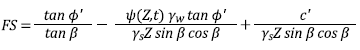
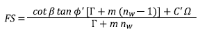
The Iverson (2000) model is a shallow landslide model that evaluates the failure of infinite slopes using an equation that balances the descending component of the motor gravitational stress with the resistance stress due to basal friction; the latter is mediated by the pressure of the water in the pores. The safety factor (FS) is calculated using equation 1.
 (1)
(1)
Where ϕ’ is the effective friction angle of the soil, β is the slope angle, ψ (Z, t) is the distribution of the groundwater pressure head, Z is the depth at which the slope fault occurs (measured vertically from the ground surface), t is the time, c’ is the effective cohesion of the soil, γw is the unit weight of the water and γs is the average unit weight of the soil.
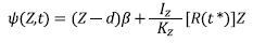
In Iverson’s model, the response of the pressure head to transient rain (in which the intensities vary during the event) is obtained from a solution in which fixed intensity and duration of rainfall are considered. In this solution, the Richards equation and superpositions of individual responses are used, as shown in equations 2-4.
 (2)
(2)
Where,
 (3)
(3)
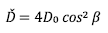 (4)
(4)
In which K z is the vertical hydraulic conductivity, d is the depth of the groundwater level measured normal to the ground surface, I Z is the intensity of the rainfall, t* is the normalized time, D 0 is the maximum characteristic hydraulic diffusivity, Ď is the effective hydraulic diffusivity and R (t*) is the response function of the pressure head that is calculated using equation 5.
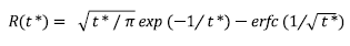 (5)
(5)
Where erfc is the complementary error function. It is worth noting that the response function, R (t*), depends only on the normalized time.
SLIP model
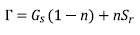
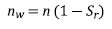
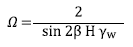
SLIP (Shallow Landslides Instability Prediction) (Montrasio and Valentino, 2008) is a model of shallow landslides that uses the infinite slope method. The SLIP model assumes that the entire amount of rainfall infiltrates the soil and that the collapse of the slope is characterized by the formation of a finite-thickness soil layer. Based on these hypotheses, the model considers that the subsoil is divided into two zones: a partially saturated overlying zone and a saturated underlying zone; the latter has a much lower permeability than the overlying stratum. The limit equilibrium method used to calculate the safety factor (FS) is shown in equations 6-9.
 (6)
(6)
Where,
 (7)
(7)
 (8)
(8)
 (9)
(9)
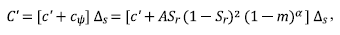
In which H is the thickness of the soil, n is the porosity, Sr is the degree of saturation, G s is the specific gravity, C’ is the total intercept of cohesion, and m is the dimensionless thickness of the saturated soil zone (ranges between 0 and 1). The total cohesion intercept, C’, is calculated from the Mohr-Coulomb failure criterion (equation 10).
 (10)
(10)
Where c ψ is the apparent cohesion related to the suction matrix, Δs is the unit length of an infinite slope section, A is a parameter that depends on the relationship between the type of soil and the peak shear stress at the fault, and α is a parameter that gives a non-linear trend to the curve that represents the function of equation 10.
The parameter m can be constant or variable over time and is correlated with the depth of infiltrated rain (h), and the volume of water required to saturate the soil; the latter is characterized by a degree of saturation S r <1. The parameter m is calculated using equation 11.
 (11)
(11)
A detailed description of the SLIP model can be consulted in Montrasio et al. (2014).
FOSM method
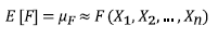
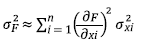
FOSM (First-Order Second Moment) is a method that uses the first-order terms of the Taylor series expansion to find the expected value, E [F], and the variance, σ2 F , of a function F (X 1 , X 2 , …, X n ), in which X i are independent variables. When the variables are uncorrelated, the statistical moments of F are calculated using equations 12-14.
 (12)
(12)
 (13)
(13)
Where,
 (14)
(14)
In which the x i are values of the variables X i that enters in the calculation of F. In this study, F is the safety factor (FS), calculated by the Iverson and SLIP models. The usual practice is to assume that the variables X i and F S are distributed according to a Normal distribution and Δx i is taken as 10% of the mean value of each variable X i (Baecher and Christian, 2003). The contribution to the variance of each variable is calculated by equation 15.
 (15)
(15)
Alternatively, the FOSM method is used to determine the probability of slip failure, PF, of slopes using equation 16.
 (16)
(16)
Where Θ is the cumulative standard normal function. The term “failure” does not refer to collapse, but refers to slope performance that does not meet expected conditions.
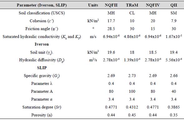
To model soil parameters as Gaussian random variables, it is required to know the mean and the coefficient of variation (COV). This last parameter is relevant because it is used as a measure of uncertainty in the characterization of soils, especially for land areas at the basin scale (Marin and Mattos, 2020). Table 1 shows the COV values established by the ISSMGE-TC304 (2021) technical committee and other researchers for parameters that are random variables in this study.
Table 1 COV of soil parameters (clays, silts, and sands).
| Soil parameter | COV (%) | Reference |
|---|---|---|
| Friction angle, ϕ’ | 4.2-12.5 | ISSMGE-TC304 (2021) |
| Cohesion, c’ | 38-51.4 | ISSMGE-TC304 (2021) |
| Unit weight, γ s | 2.6-3.3 | ISSMGE-TC304 (2021) |
| Feng and Vardanega (2019) | ||
| Permeability, K | 12.4-77.4 | Feng et al. (2019) |
In this study, the selection of the variability of the soil parameters comes from Table 1 and corresponds to a consistent analysis of the literature. It is assumed that COV (ϕ’) =10%, COV (c’) =40%, COV (γ s ) =3%, and COV (K) =12.4%. The selection of the variability of COV (K) is given to characterize the minimal effect on the Iverson and SLIP models of a highly uncertain and little-studied K parameter and its effect on FS in large areas of land.
Study site
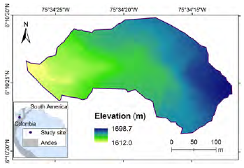
The study area is a small watershed located in the municipality of Envigado (Colombia). It is a tropical mountain terrain from the Colombian Andes. It has elevations ranging from 1698.7 to 1612.0 m.a.s.l. (meters above sea level). The location of this watershed and the digital elevation model is shown in Figure 1. The municipality has reported average temperatures of around 22°C, meaning annual rainfalls of 2170 mm, climatic classification of humid tropical forest (García- Aristizábal et al., 2019; Marín et al., 2019). Figure 2A shows the slope map of the Envigado watershed. It has slope angles above 28° (10% of the total area), with maximum slopes around 50.5°. 20% of the total area is between 15.0° and 22.4°, and 60% has slopes lower than 15.0°.
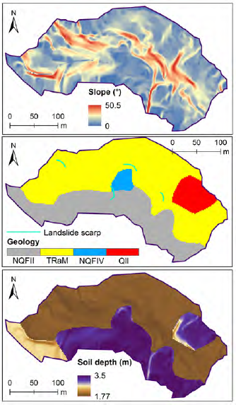
The area of the watershed is approximately 65,061 m2. Figure 2B shows the surface geological units of the watershed: amphibolites from Medellín (TraM), anthropogenic fills (QII), and two distinguished debris/mudflow deposits (NQFII and NQFIV). The amphibolites from Medellín are primarily composed of medium-sized hornblende and plagioclase feldspar series. Their texture varies between medium to fine grain sizes (foliated to massive appearance). The anthropogenic fills have a large variation in heterogeneity, including homogeneous materials conformed by technical standards for building purposes, but also with the presence of waste material (garbage), primal (or organic) matter, and loose debris materials.
The debris (NQFII) and mudflow (NQFIV) deposits are composed of gneiss (primarily), described as mildly/ moderately weathered rock fragments, with silty sand/ clay matrix. Different landslide types such as debris or planar slides, falls, and spreads have occurred in those terrains (DEACIVIL, 2015; Marin and Velásquez 2020). Figure 2B also shows the landslide scarps delimited by AMVA and UNAL (2018) in a regional landslide hazard assessment.
Parameterization
The spatial resolution of the DEM used is 2 m x 2 m (from Instituto Geográfico Agustín Codazzi, IGAC). The mechanical parameters were obtained from a geotechnical study carried out by DEACIVIL (2015), including laboratory tests. The soil effective cohesion (c’) and friction angle (φ’) were obtained from direct shear tests. The soil unit weight (γs) was calculated from natural humidity and specific gravity. These parameters were adjusted following a landslide regional study (AMVA and UNAL, 2018), where the mechanical parameters were compared with typical values for the soil types. The standard deviation for the four random variables was defined assuming coefficients of variation (COV); typical values from the scientific literature were adopted for the random input variables (Lumb, 1966; Phoon and Kulhawy, 1999) (except for Kz, proposed considering its high variability): cohesion (40%), friction angle (10%), soil unit weight (3%), and saturated hydraulic conductivity (12.4%).
The saturated hydraulic conductivity (Kz) was defined from typical values from the literature, since the spatial variability of this parameter is very uncertain and laboratory or field tests were not available. Other hydraulic parameters (D 0 , n, S r ) were also obtained analyzing the available data from the laboratory tests, but assumptions (including revising literature values) were necessary, since the data was limited. The values of λ, A, and α (SLIP model) were chosen according to the proposed values by Montrasio and Valentino (2008) for the predominant soil types of the geological units. It was assumed applicable to these soil types considering the particle sizes as the predominant characteristics of their behavior (for the selection of those model parameters). Table 2 shows the soil parameters for the two physically-based models in the Envigado basin.
The soil thickness was estimated as a function of the slope angle, and minimum values of soil thickness and slopes, as proposed by Saulnier et al. (1997):
 (17)
(17)Where zmin and zmax are the minimum and maximum soil thickness (for each geological unit), δ the slope angle, and δmin/δmax the minimum/maximum slope angles of the geological unit. According to (DEACIVIL, 2015; AMVA and UNAL, 2018), for the geological units, z min was defined as 0.2 m. z max was used as 2 m for the amphibolites from Medellín, and 3.5 for the other geological units. We considered using Saulnier et al. (1997) equation as proper for our study site since the distribution between the minimum and maximum soil depths gives higher soil depths (for lower slope angles) and tends to significantly decrease in the greater slope angles (it occurs for the tangent of the slope angle of equation 8).
The initial groundwater level was set at the soil thickness basal boundary (d lz ), as done by other researchers (Baumann et al., 2018; Kim et al., 2010; Park et al., 2013).
Results
Analysis of the spatial variation of the contribution to the variance of soil parameters
Figure 3 shows the spatial distribution of the contribution to the variance of random variables on FS of the Iverson and SLIP models. The results indicate that the parameter that has the greatest influence on the Iverson stability model is the cohesion (c’). The contribution to the cohesion variance, V (c’) = σ 2 c’/σ 2 F , ranges between 0.318 and 0.998 (Figure 3A).
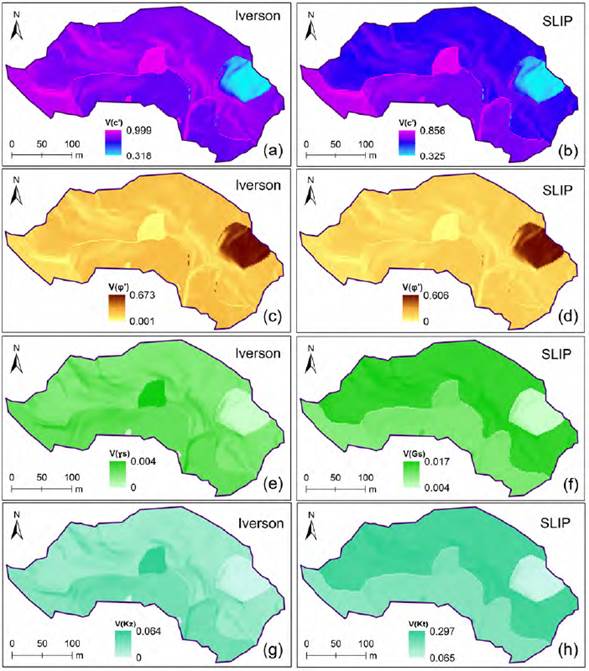
Figure 3 Spatial variation of the contribution to the variance of the soil parameters on FS of the Iverson and SLIP models.
The highest values of the contribution to the cohesion variance [V (c’) > 0.726] occur predominantly in the debris/mud flow deposits (NQFII and NQFIV), and the amphibolite from Medellín (Figure 3A and Figure 3B). In the mudflow deposits (NQFIV), the cohesive properties predominate over the frictional properties for a high soil thickness (H), and the greatest value of V (c’) is within this geological unit. In the debris/mud flow deposits II and the amphibolite from Medellín, V (c’) has a spatial variation delimited by the inclination of the slopes (β). The lowest values of the cohesion variance [V (ϕ’) < 0.202] occur mostly in anthropogenic fills, which are relatively frictional soils and are found in areas of lower slope and higher soil thickness.
Likewise, in the Iverson model, the soil friction angle (ϕ’) is the parameter that has the greatest influence after cohesion. The contribution to the variance of the friction angle (Figure 3C), V (ϕ’), reaches a maximum of 0.673 in anthropogenic fills and its variation decreases significantly [V (ϕ’) < 0.202] in areas where the cohesive properties of soils and high slopes predominate, even though soil thickness is variable. This trend is consistent with the spatial variation of V (c’).
Figure 3E and Figure 3G show that there is a wide spatial variation of the contribution to the variance of the soil unit weight, V (γ s ), and permeability of the soil, V (K), respectively. The spatial variation of both parameters is characterized by geological and topographic factors. V (K) has a greater influence on debris/mud flow deposits [0.038 < V (ϕ’) < 0.063], although it is minor compared to V (c’) and V (ϕ’). In general, in the Iverson model, the maximum contribution of the soil unit weight and hydraulic conductivity variances (combined), V (γ s ) and V (K), does not reach 7%. This result is limited by the minimal variability (10%) assumed in the FOSM method in this investigation. It reaffirms the higher effect represented by the cohesion and (to a lesser degree) the friction angle on the variation of the FS, but for all the random variables assessed in this study (c’, φ’, γ s , and K z ) their influence is conditioned by the specific geological and topographic characteristics.
As in the Iverson model, the most influential parameter in the SLIP model is V (c’) (Figure 3B), followed by V (ϕ’) (Figure 3D), and V (K) (Figure 3H). In particular, the contribution to the maximum variance of permeability, V (K), is close to 29%, and its spatial variation is controlled by geology and soil thickness. In both models, V (γ s ) (Figure 3F) and V (K) present a similar spatial variation. In the case of SLIP, the spatial trend of variances is very similar to what was seen with Iverson, although the maximum effect of V (G s ) reaches 1.73% in the amphibolite from Medellín. On the contrary, V (c’) and V (ϕ’) of the SLIP model vary according to the geology, topography, and thickness of the soil with maximum values of V (c’) = 0.856 in the debris/mud flow deposits and V (ϕ’) = 0.606 in the anthropogenic fills.
In general, in both models, the effect of the shear strength parameters on the safety factor variance depends directly on the geology and topography. In the SLIP model, there is a high spatial variance contrast of the strength parameters; that is, in an area with a high variance of cohesion, a low variance of friction occurs. This contrast is more tenuous in the Iverson model, even with equal (or very close) values of V (c’) and V (ϕ’) in some areas. In the SLIP model, the contrast is presented by the effect of the soil hydraulic conductivity. The spatial variation of the hydraulic conductivity variance is abrupt. For example, in the amphibolite from Medellín, V (K) = 0.297 is the maximum value, but in the anthropogenic fills it falls to V (K) = 0.064 as the minimum value. These results lead to the permeability uncertainty having to be characterized appropriately since an inadequate estimation could lead to inconsistent results in the SLIP model.
Analysis of the spatial and temporal variation of FS and Pf
Figure 4 shows the spatial distribution of the stability of the cells as a function of the rainfall intensity (I Z ) and duration (D). Figure 4A shows cells at the failure (FS < 1.0) and close to the failure (FS < 1.3) for the Iverson model according to relatively small intensity and duration values (I z = 0.1 mm/h, D = 1 h); while for the SLIP model, all cells are relatively far from failure (FS > 1.3). For the same intensity and duration, the distribution pattern of cells with higher failure probability (Pf) changes for the Iverson model but remains unchanged for the SLIP model. The Iverson model shows a greater number of unstable cells but also lower values of reliability index (calculated in the FOSM method, not shown as maps), causing higher failure probabilities. It can be assumed that the random variables cause more dispersion of FS (for the cells), which increases the standard deviation calculating Pf.
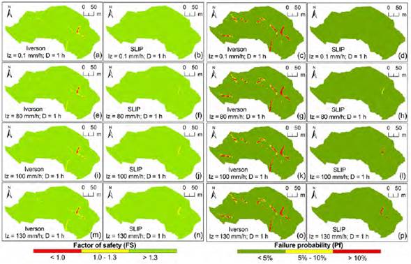
Figure 4 Spatial distribution of the stability of the cells as a function of the intensity (Iz) and duration of the rain (D = 1 h).
Figure 4 shows that for a significant increase in intensity (I z = 80, 100, or 130 mm, D = 1 h), the SLIP model slightly varies the number of cells in the failure (and close to the failure) and the failure probability.
It matches with the unstable cell areas of the Iverson model (much more unstable results), but there is a perceptible variation on the stability results (FS and Pf) varying I z (from I z = 0.1 mm to I z = 0 mm) in SLIP, unlike in the Iverson model.
Figure 4J and Figure 4L show that for a higher intensity (I z = 100 mm/h, D = 1 h), the SLIP model presents an increase in unstable cells that becomes significant for an area of high slope constituted by anthropogenic fills. Figure 4N and Figure 4P show that for even higher intensity (I z = 130 mm/h, T = 1 h), the pattern of unstable cells extends to other topographically and geologically influenced zones, although they coincide in relatively low soil thicknesses H < 2.64 m in these other zones (see Figure 2B). On the other hand, in the Iverson model, the failure patterns remain unchanged until I z = 130 mm/h.
Figure 5 shows the spatial variation of the stability of the cells for different values of intensity and duration (I z = 0.1, 80, 100, 130 mm/h, D = 2 h). The results show that the SLIP model presents greater failure areas (FS < 1.0) and failure probabilities as I z increased, compared with the 1 h rainfall event (Figure 4). Maps of rainfall intensities between 0.1 mm/h to 40 mm/h were not shown for a rainfall duration of 1 h (Figure 4) and 2 h (Figure 5), since no appreciable differences were seen (in unstable areas).
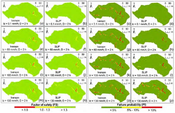
Figure 5 Spatial distribution of the stability of the cells as a function of the intensity (Iz) and duration of the rainfall (D = 2 h).
In this case, the increases in the failure probability in the SLIP model are regarded to the sensitivity of the FS to the thickness of the unsaturated layer, the variation of the shear strength parameters, and the permeability of the cells with a steep slope gradient. In contrast, the failure patterns of the Iverson model remain practically invariant for different rainfall intensity values (I z = 0.1 to 130 mm/h) and D = 2 h. In terms of Pf, the shallow landslide-prone areas are similar in both models for the most extreme rainfall intensity (130 mm/h). Again, the Iverson model presented instabilities or higher Pf values starting from the very low intensity (I z = 0.1 mm/h) scenario with very little (or no) variation as I z increased. The SLIP model showed more progressive instabilities as I z increased (at least for higher I z values).
Figure 6 shows that the spatial distribution of the unstable cells in the Iverson model increased marginally for a rainfall duration of 4 h (compared with shorter durations). The FS decreased as rainfall intensity increased even with the lower intensity values that were simulated (slight variations are noticed for Iz = 10 mm/h and 20 mm/h). For SLIP, the difference in the distribution of FS and Pf is little when comparing the smallest event (I z = 0.1 mm, D = 4 h) with rainfalls of shorter duration. Failure was not reached for any cell and Pf values were lower than 10% (with a very small area with values between 5% and 10%) for intensities lower than 20 mm/h. With increasing rainfall intensity for D = 4 h, the SLIP model yields a considerable increase in the area of unstable cells and greater Pf. For D = 4 h, the Iverson model presented no appreciable variations for the longer intensities (not presented in the figure); the SLIP model presented increasing instability as the intensity increased. Unlike in the shorter rainfall events, in this case, the SLIP model caused greater unstable areas than the Iverson model (for the high-intensity rainfall events).
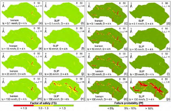
Figure 6 Spatial distribution of the stability of the cells as a function of the intensity (Iz) and duration of the rain (D = 4 h).
Figure 7 shows that the Iverson and SLIP models presented very similar stability results (when D = 8 h) after different 60 and 100 mm/h, respectively. The Iverson model presented increases in the spatial distribution of unstable cells with the intensity variation from I z = 0.1 to 60 mm/h, but from I z = 60 to 130 mm/h the results were invariable. The SLIP model presented a similar behavior after I z = 100 mm/h. As was seen for the event of D = 4 h, the SLIP model presents higher unstable and greater failure probabilities than the Iverson model, in this case requiring lower intensities than for shorter rainfall duration events.
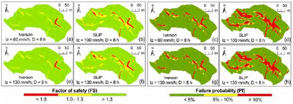
Figure 7 Spatial distribution of the stability of the cells as a function of the intensity (Iz) and duration of the rainfall (D = 8 h).
Figure 8 shows that when D = 16 h, the behavior of both models shows an increase in the failure area as the intensity increases. Interestingly, the tendency that appeared to stabilize the SLIP model and would present greater unstable areas for longer and more intense rainfall events, did not continue for this longer event. In the Iverson model, the distribution of cells near to the failure (and even the failing cells, slightly) is greater than in the SLIP model. Regarding the distribution of unstable cells, in both models, they are similar up to I z = 20 mm/h, from which in the SLIP model the number of cells failing increases noticeably up to I z = 60 mm/h. Even though the constituted by unstable cells of the SLIP model coincides for the most part with the area conformed by failing cells (or close to the failure) of the Iverson model, there are some unstable areas in SLIP that are stable in Iverson, and vice versa.
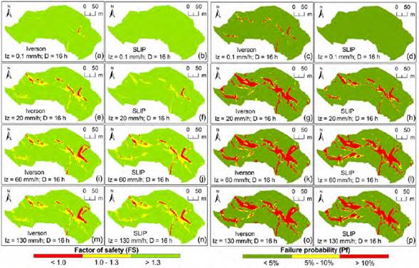
Figure 8 Spatial distribution of the stability of the cells as a function of the intensity (Iz) and duration of the rainfall (D = 16 h).
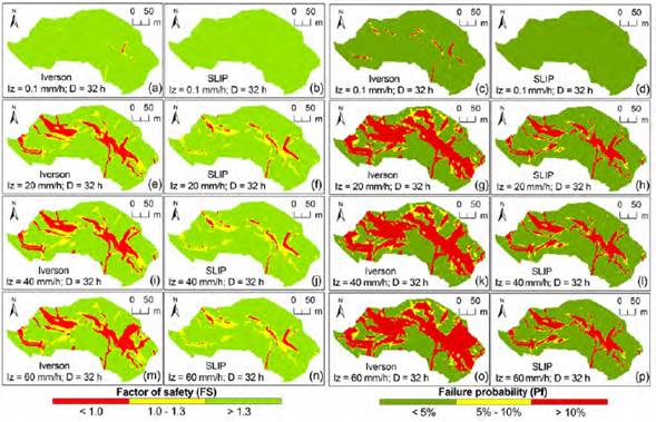
For D = 32 h, Figure 9 shows that both models present the largest spatial distribution of failing cells and greater failure probabilities even for a rainfall intensity of I z = 20 mm/h. The instability is considerably higher in the Iverson model, which stabilizes (no significant variation in the stability results) after I z = 60 mm; while SLIP stabilizes after I z = 40 mm/h (in terms of the intensity scenarios simulated).
Discussion
The topographic, geological, and soil thickness factors have a high influence on the contribution to the variance of the soil properties. The results showed that in the Iverson and SLIP models, shear strength parameters have the largest contribution to variance, while permeability and soil unit weight (or specific gravity) have a minor effect. It does not mean that the variables do not affect landslide occurrence. It indicates that small variations of those parameters (under the actual conditions of our study area) cause a minor variation in the effect of safety and failure probability.
Several authors have established the significant effect of mechanical and hydraulic properties on slope stability (Marin and Velásquez, 2020; Wang et al., 2020; da Silva et al., 2021; Materazzi et al., 2021). Listo et al. (2021) used the TRIGRS model in a basin located in The Serra do Mar Mountain Range (Brazil), simulating two scenarios which allowed them to verify that the model is very sensitive to cohesion and soil depth (besides the water table, which was well recognized by other authors, stated also in the TRIGRS manual). It was also expected for the infinite slope stability models used in our research work. Nevertheless, more specific details reported about the variation of this effect depending on the soil depth or slope angle (also for the other parameters such as friction angle or soil unit weight), makes that our results have significance for the scientific community. Interestingly, different surface failures such as slope-parallel planar surfaces (infinite slope stability model), a succession of rigid bodies of infinite width (Janbu’s model), or ellipsoidal sliding surfaces modeled by r.slope.stability (Mergili et al.. 2014) allowed Zieher et al. (2017) to conclude that the influence of cohesion decreases (non-linearly) as soil depth increases. In our study, the soil depth was calculated as an inverse function of the slope gradient so that it is not completely clear that the dependence of the cohesion (or any other parameter analyzed in this research) is directly related to the variation of the soil depth or slope angle (specifically).
The maximum contribution that permeability and unit weight together made to the variance did not exceed 7% of the whole study area. In contrast, in the SLIP model, only permeability has a contribution to the maximum variance close to 30%, with an even greater contribution from cohesion and friction angle in most cells. Future implementations of the SLIP and Iverson models should take into consideration a proper characterization of the mechanical soil properties (mainly the soil effective cohesion), but knowledge about the soil type (e.g. cohesive or frictional soil), slope angle, or soil depth, can help us to get an idea of the effect of the variation of the random variables (studied in this research: c’, φ’, γs, and K z ) on the factor of safety results.
The results showed that, although the Iverson model was (apparently) more conservative before rainfall or for negligible rainfall intensities (Iz = 0.1 mm/h), it was less sensitive to rainfall intensity than SLIP in shorter durations. For events longer than 8 h, the Iverson model was very sensitive (FS and Pf varied with intensity) and disastrous (many more unstable cells and higher failure probabilities). In the range of 4 to 8 h, an unpredicted behavior occurred since the SLIP model had more unstable areas than Iverson for most of the intensities simulated.
In general, the spatial variation of the unstable cells (or higher failure probability) as a function of intensity and duration for both models did not allow to establish absolute tendencies in general terms about the more conservative. Specific conditions were identified that can serve to understand the behavior of the models for short or long rainfall events and low or high-intensity events. The Iverson and SLIP models respond in different ways to the variation of rainfall conditions: for shorter durations (e.g. ≤ 8 h), increasing the intensity caused more unstable areas in the SLIP model, while for longer durations the unstable areas were considerably higher for the Iverson model. In all cases, a maximum failure area is reached so that a more intense event (for a specific duration) will not cause more unstable grid cells. Understanding those behaviors can be useful for its implementation on landslide prediction or forecasting, landslide susceptibility, hazards or risk assessment, and even further implementations in methodologies to define rainfall thresholds.
Conclusions
In this research study, the first-order second-moment (FOSM) method allowed calculating the contribution of the effective cohesion, effective friction angle, unit weight, and saturated hydraulic conductivity to the variance of the factor of safety two distribute slope stability models (SLIP and Iverson). In general terms, cohesion has the largest contribution to the variance of the FS, which indicates that a small variation on this parameter has a greater effect on the FS results. Nevertheless, the magnitude of this variance varied on different geological units and slope angles/soil depths. Those variations occurred for all the random input variables analyzed. It suggests that the magnitude of the specific variable (e.g. cohesion) also affected that a small or great variation of this parameter has a minor or greater effect on the FS and failure probability results. The Iverson and SLIP models respond in different ways to the variation of rainfall conditions. Understanding those behaviors can be useful for practical and appropriate implementation of the models in landslide assessment projects.
The implication of the differences in the models is relevant for application in an early warning system based on rainfall thresholds, landslide zoning, among others. Therefore, it is advisable to characterize models assuming different analysis conditions for a specific study site where it is being implemented or where a potential application is projected. Future studies could assess the effect of the random input variability on the slope stability under the different rainfall scenarios (short/long durations and low/high intensities). Also, the uncertainty of the input parameters may be incorporated and assessed with probabilistic methodologies (e.g., Monte Carlo simulation). The predictive capacities of the physically-based models considering the distribution function of input variables can be evaluated by calibrating the input data through back-analysis of real landslide events. In those cases, the sensibility of the models can be also verified since most of the model validations in the scientific literature do not consider the possibility of erroneous predictions derived from minor variations of the input parameters (even for probabilistic assessments).

