


 Inglês (pdf)
 Artigo em XML
 Referências do artigo
 Enviar este artigo por email
 Citado por SciELO
  Citado por Google
  Similares em
SciELO
Similares em
SciELO  Similares em Google
 Permalink
1. Introduction
In recent years, air pollution has been extensively studied, due to its economic and health consequences, especially concerning the fine particulate matter with 2.5 microns diameter (PM2.5) [1]. Some authors [2-4] have reported a relationship between meteorological conditions and the levels of contamination reached at specific periods. These levels of pollution are derived from the values of certain atmospheric variables. In particular, three variables seem to be directly related to contamination: horizontal wind, which disperses pollution, atmospheric stability, which determines vertical air motions that can reduce the concentration of pollutants, and precipitation, which dilutes pollutants and drives wet deposition [5-8]. Consequently, studying these factors can be useful for understanding the variation and dispersion of PM2.5 in tropical Andean megacities. Most research has been based on simulating pollutants[9-12], studying their chemical composition [13,14], and determining their sources of emission [15]. However, it is essential to investigate the behavior of PM2.5 linked to local meteorology, as some studies [16,17] have found that atmospheric patterns account for more than 20% of the variation of the PM2.5, e.g., due to the atmospheric characteristics;[18] reported that both surface roughness and atmospheric stability are the main control factors of particle deposition, alongside particle diameter, which was also described by [19]. Therefore, stability seems to be one of the most important variables regarding pollutant dispersion. From the findings of other authors[18,19], we can identify the importance of studying in greater depth the relationship between stability and PM2.5, especially in tropical cities (where atmospheric dynamics are not fully understood).
Several authors have studied the relationship between the meteorological conditions of a place and pollution. [20] established statistical relationships between PM2.5 and atmospheric patterns to create methods to control the pollution levels, they used multiple linear regressions to determine how PM2.5 is related to temperature and precipitation, finding that temperature could be related to PM2.5 concentrations, and the area, due to the production of thermal inversions and/or vertical velocity. [21] used a Geographically Weighted Regression to understand the meteorological behavior and its relation to the area and pollution. They reported that the terrain and fluxes are important to describe pollutant variations. On a larger scale, [22] studied the relation of synoptic weather conditions presented in highly polluted events, they found that wind speed is important for pollution dispersion. For example, in Seoul, the reduction in pollution levels was not caused by policies but also produced by changes in local meteorology, especially in terms of wind speed changes. This phenomenon was also studied and reported by [23]. Other studies were also conducted for variables such as precipitation, radiation, relative humidity, and Boundary Layer Height (BLH) [24-26].
One different approach was executed by[27,28]. Both studies focused on composites analysis of meteorological variables to improve the comprehension of PM2.5 trends and variations. These and other subsequent studies [29-31] determined that linking the meteorological variables associated with a specific area to pollution could improve the forecast of high pollution events. Focusing on this approach (i.e., composite analysis), some authors [31,32] identified that wind field, precipitation and BLH are the variables that produce movement of air (i.e., dispersion) and also stagnation. For this reason, they created an index of stagnation to determine the probability of an increase in contamination due to meteorological patterns presented in a given area.
In the tropics, atmospheric stability has been mainly studied for meteorological purposes. [33] concluded that there is a close relationship between the development of turbulence in the boundary layer and the formation of deep convection in the atmosphere. The former elucidates the significance of the link between the mixing layer and air rises and, thus, atmospheric pollution. One of the first approaches to study the relationship between stability and particulate matter in the tropics using radiosonde data was made by [34], identifying that fire events cause highly polluted events. This explains (and raises the question of the importance of wind direction in the increase of PM2.5 concentration in the city of Bogota) a fraction of the amplitude of PM2.5. On the other hand, the remaining fraction is caused by the height of the mixed layer and, therefore, stability. Hence, evaluating the behavior of the components that determine the height of the mixed layer and its relationship with particulate matter is paramount [35]. All of the aforementioned studies increase our understanding and comprehension of the behavior of particulate matter and, thus, serve as a basis for what must be taken into account in air pollution models and parameterizations.
Although some studies have focused on the relation of meteorological variables and contaminants, only a few have investigated the stability in a tropical megacity with a complex terrain such as Bogota and include more than four meteorological variables. Bogota [Figure 1] is a tropical megacity with specific orographic characteristics. It is important to highlight that, in Bogotá, industries and mobile sources currently emit a significant percentage of the pollutants. The city also has an air quality monitoring network (AQMNB - Air Quality monitoring Network of Bogota) with 12 stations and a daily radiosonde, carried out at El Dorado Airport at noon.
Therefore, Bogota was selected as the study area allowing the evaluation of the atmospheric conditions: air temperature, radiation, relative humidity, wind direction, wind speed and its components, BLH, Turbulent Kinetic Energy (TKE), and atmospheric stability present during a pollution event in a mountainous area of the tropics. [34] (based on our information, this is the first study to focus on the relationship between stability and air pollution in the Andes Mountain range), carried out an approach to the study of stability and the boundary layer in relation to particulate material. However, the cited study did not consider the detailed description of the atmosphere behavior in episodes of high and low concentrations of PM2.5. Consequently, this article aims at determining and analyzing the most important atmospheric characteristics present when there is a highly polluted event in a tropical city.
2. Method
2.1. Data
Data retrieved correspond to the variables: solar radiation, air temperature, wind speed and direction, relative humidity, and PM2.5. Surface observed data was retrieved from the AQMNB stations between 2013 and 2020 with a temporal resolution of 1 h [Figure 1] [36], the data have already been checked by [36], but here we also follow the quality control done by [37] to increase the data reliability. The stations that have more than 75% of valid data are used. Daily data (12:00 UTC) of radiosonde station 80222 Reported by the University of Wyoming (http://weather.uwyo.edu/upperair/sounding.html) was also used in this study in the analysis of stability through the comparison of skew-t diagrams available online. Additionally, a reanalysis database (ERA-5) of vertical velocity and boundary layer height with a temporal resolution of 1 hour and a 0.25º of spatial resolution between 2013 and 2020 was used for the performance of the analyses [38]. The vertical velocity data has been validated by [39], and the boundary layer height has been used and evaluated by [40].
2.2. Episode selection
To perform the analyses, the daily Air Quality Index (AQI) [41] was used to select the days between 2013 and 2020 with the characteristics to be considered polluted or not. The days with AQI values between 100 and 200 were classified as Polluted days (PD) and the days with values from 0 to 50 as Non-Polluted days (NPD), days with intermediate AQI (50 to 100) or higher than 200 were omitted since they are not extreme values [Table 1] [Figure 2]. As a reference, the methodology proposed by [12] was used.

2.3 PM2.5 daily variation
Initially, PM2.5 concentrations for the city can be analyzed by their daily variation during PD and NPD, as defined above. The PM2.5 concentration has higher values during the PD than during NPD for the whole day [Figure 3]; this fact validates the selection of the PD as a set of studies. Pollutant concentration values have a larger standard deviation during PD than during NPD. PM2.5 peaks during the morning hours, reaching its maximum at 8h and 9h. After 11h, the pollution levels are rapidly reduced, in both PD and NPD; this can be caused by the wind field's daily variation, which leads to strong dispersion caused by either dynamic horizontal advection (i.e., horizontal dispersion dominates) or vertical air motions. These possible causes will be studied in the following sections.
2.4 Atmospheric stability and PM2.5 concentrations
To analyze the relationship between stability and PM2.5 concentration, two different methods were used:
1) The Pearson, Kendall, and Spearman approach for linear correlation were calculated between CAPE (Convective Available Potential Energy) and CIN (Convective Inhibition) indexes, and PM2.5 concentration [Table 2] [42,43]. This approach uses the absolute values of CAPE and CIN for the linear correlation with the PM2.5 concentrations, since CIN is the inverse value of CAPE, the use of the absolute values for both indexes allows characterizing the relationship between a stable atmospheric condition and the pollutant concentration.
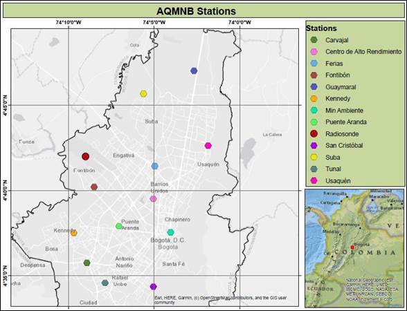
Figure 1 Map of the study area. The dots represent the location of the AQMNB (Air Quality Monitoring Network of Bogota) stations, and the red cross indicates the location where the radiosonde is sent
Figure 2 Temporal distribution of the AQI (Air Quality Index) in the city between 2013 and 2020, and identification of the Polluted days (PD) and Non-polluted days (NPD)
2) An analysis of thermodynamic diagrams (Skew-t) was performed since it allows determining the stability of the selected episodes. This approach takes into account whether the atmosphere is unstable, stable, or neutral, and detects the presence of thermal inversions, two important characteristics of tropical meteorology. To analyze the Skew-t, the parcel method was used; it is based on the adiabatic rise of an air parcel so that its temperature changes as it expands/compresses, as it moves in the atmosphere[44]. With it, it is possible to describe the stability of the atmosphere in the identified episodes of high and low pollution.
2.5 Turbulent kinetic energy and PM2.5 concentrations
A study of the microscale atmospheric variables trends was conducted, considering specifically the variables: air temperature, radiation, relative humidity, wind speed and wind direction, boundary layer high, wind components (u, v, w), and the Turbulent Kinetic Energy (TKE).
Table 2 Correlation benchmarks for the Pearson, Kendall, and Spearman coefficients calculated between atmospheric stability, CAPE (Convective Available Potential Energy), and CIN (Convective Inhibition), with PM2.5 concentration
The TKE (Equation 1 (TKE per unit mass)) is one of the most important variables in micrometeorology [35], since it is linked to the intensity of turbulence, it also gives an insight into pollutants mixing in the atmosphere (e.g. [35]). In Equation (1), u, v, and w are the zonal, meridional and vertical components of the wind in ms-1, respectively.
To perform the analysis, composites of each variable were calculated for the entire period (2013-2020) and the PD and NPD. The composites analysis aids in the process of identifying differences between atmospheric conditions and allows identifying important relationships between pollution events and meteorological variables (e.g., [44,45]).
3. Results and discussion
3.1 Atmospheric stability and PM2.5 concentrations
This section presents the statistical correlation between the atmospheric stability condition (based on the CAPE and CIN indexes) and PM2.5 concentration using the Pearson, Kendall, and Spearman approaches. Figure 4 shows the values of the correlation coefficients computed with the mentioned statistical approaches sorted by PD and NPD. The correlation coefficients for the PM2.5 concentration and the atmospheric stability condition based on the CAPE index [Figure 4 Top) have values between -0.13 and -0.42 for PD (i.e., No correlation to Negative Moderate correlation). Similarly, the correlation coefficients for the PM2.5 concentration and the atmospheric stability condition based on the CIN index [Figure 4 Bottom) have values between -0.13 and -0.47 for PD (i.e., No correlation to Negative Moderate correlation). This means that the relationship between the atmospheric stability and the concentration of PM2.5 trends to be negative and weak during PD.
Considering the results for NPD the correlation in Figure 4, the stability evaluated through CAPE got values from -0.02 to 0.036 (i.e., No Correlation). For CIN, the correlation regarding the NPD got values from -0.04 to -0.134 (i.e., No Correlation). This means that during NPD, the relationship between atmospheric stability and pollution levels is undetermined.
Figure 4 Correlation coefficients between the atmospheric stability and PM2.5 concentration of the PD and NPD composites: CAPE (Top) and CIN (Bottom). A positive correlation corresponds to a high PM2.5 concentration and a stable atmospheric condition
These results show that initially convective atmospheric instability does not reduce PM2.5 levels over Bogota since CAPE and CIN are linked only to convection potential. Even so, the mean P-value during NPD and PD was 0.28 and 0.065, respectively, showing that the significance of the statistical results is still low and therefore insufficient to make conclusions regarding the relationship between atmospheric stability and PM2.5 levels based on the CAPE and CIN indexes over Bogota.
To fully understand how vertical motions interact with the pollutants over Bogota, an analysis of atmospheric diagrams (parcel method) as a complementary approach for every day is performed for both PD and NPD. This analysis is based on the Radiosonde data retrieved from the University of Wyoming Website.
Figure 5 Percentage of repartition of atmospheric phenomena during PD and NPD. The phenomena used for the classification were: W/OTI: % of days without thermal inversion, WTI: % of days with thermal inversion, NS: % of days with neutral stability, W/OS: % of days without stability, and WS: % of days with stability
The results of the skew-t diagrams analysis are summarized in Figure 5, where PD and NPD are shown separately. The different phenomena identified are W/OTI: % of days without thermal inversion, WTI: % of days with thermal inversion, NS: % of days with neutral stability, W/OS: % of days without stability, and WS: % of days with stability. To better describe the data, it must be considered that: W/OTI + WTI = 100%, and NS + W/OS + WS = 100% for PD and NPD separately.
The results in Figure 5 show that the atmosphere over Bogota is mainly stable (WS ﹥ 50%, and WTI ﹥ 80%), or neutral (NS ﹥30%). Additionally, PD and NPD have the same proportion of stable and neutral stable days. In contrast, W/OS ﹤ 13%, and W/TI ﹤ 15% for PD and NPD are evidence of the high atmospheric stability of the city. These results are coherent with the evidence collected from the first approach [Figure 4], leading to identifying that vertical motion is not linked to the dispersion of pollutants in the city.
The atmosphere has thermal inversions in more than 85% of the cases (PD and NPD); this leads to evidence that Bogotá normally presents atmospheric inversions and other forms of stable atmospheric conditions, but this is not linked to pollution levels in the city.
Therefore, these findings support the argument that vertical air motions do not have an important relationship with the variation of PM2.5 concentrations of Bogota, and indicate that other dynamical phenomena such as TKE [35] , wind speed [23], or wind direction may have a stronger effect on pollution dispersion in Bogota.
3.2 Relationship between local meteorology and PM2.5 levels during polluted days
This section presents the analysis of the temporal variation of local meteorology variables and its relationship with the PM2.5 levels during PD and NPD. Hourly average time series of wind speed, wind direction, air temperature, radiation, relative humidity, wind components (u, v, w), the height of the boundary layer, and the TKE were calculated. The presented profiles were calculated with the average of all the stations of AQMNB.
Radiation, temperature, and relative humidity
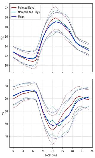
Figure 6 shows the hourly average solar radiation profiles sorted by PD and NPD. The radiation starts increasing at 7h, with a peak of radiation at 12h. Thereafter, radiation decreases until 19h. Higher average radiation is observed for PD than for NPD between 9h and 14h. Since radiation correlates to air temperature, this peak can also be observed in the air temperature variable shown in Figure 7 (Top). This peak in radiation is explained by the season of the year in which the PD takes place since most of the PD occurs between February and March, a high radiation season in Colombia. March is the month associated with fire events in Colombia. This matches the results of [34] that relate highly contaminated events to fire events in Colombia, specifically, near Bogota during February and March.
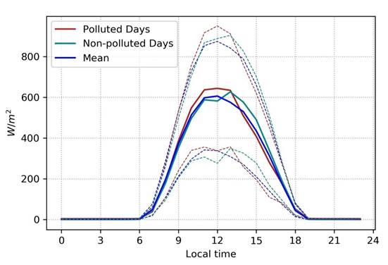
Figure 6 Hourly average profile of Solar Radiation. Continuous lines represent the hourly average values of the variable over the city. Dotted lines show the ∓ standard deviation of the averaged values
Air temperature on PD [Figure 7 Top) is lower than for NPD until 7h. Then, it has a rapid increase that reaches higher values than the NPD. After the temperature peaks around 14h, a rapid decrease in this variable is evidenced, which leads to a considerable increase in relative humidity on PD (i.e., half standard deviation). In summary, the temperature peak on PD is higher than normal and then decreases rapidly, leading to higher humidity values after 12h.
Wind field
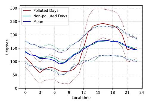
Wind direction [Figure 8] and wind speed [Figure 9] are important variables to analyze in conjunction, as the former can bring pollution from external sources (e.g., wildfires, biogenic aerosols, or Saharan dust), and the second can disperse the contaminant through advection phenomenon. The wind during PD blows mainly from the east (normally, it comes from the southeast). The northeast of Colombia is characterized by the large plains and the Orinoco Basin [Figure 1], an area between Colombia and Venezuela, where an important part of the wildfires of the Region occurs, especially between February and March [46]. The pollutants emitted from this combustion source are then transported to Bogota, increasing pollution levels as reported by [34]. This pattern of wind direction coupled with low air temperature (and low BLH) and slower wind speed (in the morning) leads to an increase in pollution levels in Bogota.
The wind direction has a rapid change after 11h, passing from easterly winds to southwest winds, which means that the zonal component of the wind changes more drastically than its meridional counterpart. This behavior is not found in the mean or NPD. Wind speed in the morning hours of PD is lower in comparison to NPD (one standard deviation). Around 11h, there is a rapid change in the wind speed trend, only present in PD. Additionally, on NPD, wind speed is higher than the average, between 7h to 12h. The latter indicates that this variable may be relevant for changes in pollution levels. This observation is evidence of a process in which easterly winds bring pollution from the eastern plain wildfires into Bogota during the morning of PD as it has been already observed in published works (e.g. [46,47,34]) and thereafter, the wind drastically changed its direction. After 12h, the pollution level decreases due to wind speed and temperature increasing patterns (i.e., a decrease in PM2.5 may be associated with TKE and the BLH).
Boundary-Layer Height (BLH)
The effect of the BLH in atmospheric pollution is documented as inverse since it can reduce the pollution levels when it increases [48]. However, it is necessary to consider two variables with a large influence on the BLH: temperature and TKE [35,49]. Air temperature results are important since it has an expansion effect on the BLH; TKE can increase BLH due to wind shear. The final effect of BLH is to increase pollutants dilution on the surface, therefore reducing pollutant concentrations.
According to the results obtained for the radiation [Figure 6] and temperature [Figure 7 Top), BLH is expected to be lower in the mornings on PD than during NPD [34]. BLH is also expected to increase during the afternoon, reaching values larger than during NPD [Figure 10]. In other words, during the morning, BLH is slightly lower in PD than in NPD but then increases during the afternoon (with the increase in air temperature), and its peak is half standard deviation higher than the mean. This means that BLH, and therefore pollution levels, are sensitive to daily thermal changes.
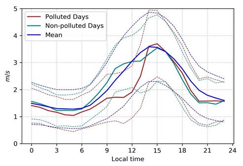
Figure 9 Hourly average profile of wind speed. Continuous lines represent the hourly average values of the variable over the city. Dotted lines show the ∓ standard deviation of the averaged values
However, the differences between PBH for PD and NPD during the mornings are not significant, indicating the importance of the shear component in the variation of PM2.5 concentration, as was also reported by [50].
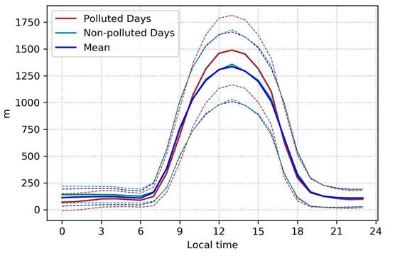
Figure 10 Hourly average profile of Boundary Layer Height (BLH). Continuous lines represent the hourly average values of the variable over the city. Dotted lines show the ∓ standard deviation of the averaged values
Accordingly, the shear that depends on wind components (u, v, w) is evaluated and reflected on the TKE [Figure 11]. Before describing the behavior of wind components, it is important to mention that the magnitude of u and v depends on the wind direction since wind is a vectorial field. Thus, if the wind direction changes, the magnitude of u and v will change. To better understand the components, first, we evaluated the w-component (vertical wind velocity component) on PD, w has higher values from 0h to 15h, a consistent observation with the results reported in previous sections [Figure 4 and Figure 5], where the vertical motions are not linked to pollution levels reduction.
The local u-component on PD is stronger during the entire day, but especially between 12h and 18h, due to a rapid increase in its trend (i.e., an increase in its magnitude and the change in wind direction). The aforementioned matches the results from the wind direction and speed [Figure 8 and Figure 9], implying that the u-component carries the smoke from the eastern plains of the Orinoco basin (possibly wildfires) to the city in the morning. The meridional (v-component) has lower values in PD than the Mean and NPD throughout the entire day, especially between 9h and 10h (almost one standard deviation). Additionally, the v-component of the wind presents the same rapid increase (the steeper growth is due to the magnitude and not the change in direction, which is not significantly large for the meridional component) in the afternoon, similar to what is observed in regards to the local u-component.
After describing the components of the wind, TKE is analyzed due to its possible importance in pollutant dispersion over the city. When TKE presents high values, there is an increase in turbulence and boundary layer height and, hence, the mixing and pollutant dispersion is greater [34,35]. This implies that pollution concentration decreases when TKE increases. Additionally, TKE on PD in comparison to the Mean and NPD is lower during the day, especially between 10h and 13h (at 12h, the TKE is around half a standard deviation lower). Between 13h and 15h, the TKE has a rapid increase (also perceived in wind speed and its components). Thus, during the morning of PD (from 9h to 13h), there is less dispersion and mixing of pollutants. Accordingly, the variable with a larger influence on the concentration of PM2.5 is the TKE (which mainly depends on the horizontal components of the wind because of its magnitude). Note that the u-component has the least correlation among wind components.
3.3 Local meteorology and PM2.5 concentrations
This section describes the significance of local meteorology with PM2.5 concentrations during PD, to quantitatively identify the relationships between them. Of the 10 variables (Radiation, Air Temperature, Relative Humidity, Wind speed, Wind direction, BLH, u-component, v-component, w-component, and TKE), only 3 have a statistical significance [Table 3]: radiation, wind direction, and the v-component of the wind. Radiation has a moderate positive correlation with PM2.5, meaning that if radiation rises, PM2.5 also increases.
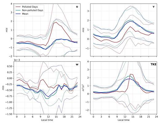
Figure 11 Hourly average profile of u-component (Top left), v-component (Top right), w-component (Bottom left), and TKE (Bottom right). Continuous lines represent the hourly average values of the variable over the city. Dotted lines show the ∓ standard deviation of the averaged values
This behavior could be explained due to radiation energy rising the number and speed of chemical reactions that produce secondary aerosols sensed by the AQMNB as PM2.5. Likewise, the high values of radiation match with the largest number of wildfires that occur in Colombia and Venezuela, and with the season of the year when most of the high pollution events occurred.
Wind direction has a moderate negative correlation. However, it is important to carefully evaluate this result. Low values (between 50 to 100) are from the east; therefore, the wind is coming from the eastern plains, the place where most of and the most intense wildfire events occur [46,47,34]. When the wind changes its direction (e.g., to the southwest), the smoke is reduced due to fewer wildfires (e.g.,47,50]. The v-component of the wind has a moderate negative correlation since this component has lower values at 9h and after 12h increases. The aforementioned behavior is the opposite of what happens on PD, where the PM2.5 has its peak at 9h and 10h and then decreases.
Air quality is strongly linked to meteorology and emissions. Different interactions between these three elements (air quality, meteorology, and emissions) may affect air pollution with different intensities and at different scales. In this study, we observed that, at the regional scale when regional pollution is transported and present in the upper layers, the vertical mixing does not reduce importantly the city’s air pollution; in contrast, at the local scale when the upper layers are clean (i.e., small presence of regional pollution), local pollution is mainly linked to local emissions, therefore, when the near ground polluted air layers are mix with cleaner air from upper levels, reducing surface pollution levels.
4. Conclusions
Bogotá has a large risk associated with PM2.5 on a yearly, daily and hourly time scale [51]. Different phenomena are related to these PM2.5 variations and their understanding helps to complete already published research. For this, the relationships among PM2.5 concentrations, local meteorology variables, and atmospheric stability were evaluated in this study. Specifically, the relationship between wind field, TKE, radiation, temperature, relative humidity, BLH, and atmospheric stability (i.e., CAPE and CIN) with PM2.5 concentration was quantitatively investigated.
Table 3 Correlation between local meteorology variables and PM2.5 concentration over the city of Bogota during PD between 2013 and 2020
Statistical correlations (Pearson, Kendall, and Spearman) and the parcel method were used to analyze the relationships between atmospheric stability, vertical air motions, and PM2.5 concentrations, leading to conclude that the stability does not affect the concentrations of PM2.5 significantly. The stability indexes evaluated (i.e., CAPE and CIN) have little or no correlation with PM2.5 concentrations according to the evaluation criteria established. A similar lack of correlation is observed for the parcel method results. Therefore, neither atmospheric stability nor thermal inversions influence the variation of PM2.5 concentration. This implies that vertical air motions do not significantly influence the surface pollutant concentration.
Hourly composites of the meteorological variables were made, resulting in wind speed, wind direction, radiation, meridional wind (highest relation), and the TKE being associated with changes in the trend of pollution. A statistical test was also performed to find the statistical correlation between the meteorological variables and PM2.5. These analyses lead to conclude that solar radiation is more intense during PD than during NPD, a key observation since it is related to external sources based on wildfires, and intensifies the chemical reaction kinetics responsible for secondary aerosol formation and therefore PM2.5 levels.
During PD, the air temperature is low during the morning and high during noon in comparison to NPD. Temperature profiles correlate with BLH changes since it is sensitive to diurnal thermal variations. BLH is lower in the morning but higher throughout the rest of the day, during PD and NPD, which coincides with the diurnal temperature variation, i.e., BLH variation is linked to diurnal temperature variations, but it is not linked to the horizontal advection present in the afternoon. This may indicate that BLH variation (and diurnal temperature variation) is not closely related to the concentration of PM2.5.
The wind blows from the east in the morning during PD. These winds transport pollutants from the Colombian-Venezuelan plains. These pollutants are produced during combustion in the wildfires that commonly take place in February and March. During PD, the PM2.5 is not effectively dispersed because the wind speed is slower (almost one standard deviation) than normal, especially between 10h to 13h. In the afternoon, the wind direction changes, and the speed rapidly increases. This is not evident in the NPD. Hence, dynamic field perturbations in the wind are essential in the variation of PM2.5 during PD. For this reason, dynamic fields associated with the wind are essential to simulate, and one new approach that has produced good results is described in [52].
The v-component [Figure 11] of the wind is low during the day and increases after 14h when the PM2.5 concentration also decreases (this also occurs with the u-component). Thus, the meridional wind seems to be the most related to PM2.5 variation (alongside wind direction). A feature that is also observed for the TKE, which is considerably linked to pollution, the aforementioned can be explained by the fact that turbulence energy allows for mixing to occur and, hence, pollutant dispersion takes place. A result that contributes to the explanation of the PM2.5 concentration being higher in the morning than in the afternoon since the TKE is two times larger at 18h (1.3 m/s) than at 8h (0.3 m/s). Consequently, it is important to further investigate the TKE in idealized physical models to improve our understanding of this variable and its relation to PM2.5.
In general, our results point toward three strong atmospheric conditions linked to high PM2.5 concentrations: i) horizontal wind speed and TKE throughout the day weaker than during a mean day o NPD, ii) easterly winds in the morning (associated with the transport of pollutants from wildfires produced on the Eastern plains) (e.g., [53]), and iii) solar radiation peaks higher than during a mean day of NPD, these atmospheric patterns lead to the detrainment in Bogota’s air quality.

