


 Inglês (pdf)
 Artigo em XML
 Referências do artigo
 Enviar este artigo por email
 Citado por SciELO
  Citado por Google
  Similares em
SciELO
Similares em
SciELO  Similares em Google
 Permalink
1. Introduction
Chemically reacting flows have several applications in engineering [1-10]. To accurately solve chemically reacting turbulent flows is a current challenge of the Computational Fluid Dynamics (CFD). It is known that a direct numerical simulation (DNS) is the best tool for the analysis of It allows solving the whole range of spatial and temporal scales of turbulence without being necessary to implement turbulence models. But this technique, at least for now, is out of reach for all engineering applications [11-18]. The large eddies simulation (LES) technique, developed relying on the spectral filtering of the turbulent energy, is a better form of dealing with turbulence normally found in engineering applications [19-21]. The most suggested type of filtering implies the decomposition into different zones of the energy spectrum, starting from a wave number k c the grid size ∆ can be successively used as a cutoff filter while the wave number remains lower than another wave number k d , previously selected at the far end of the spectrum. The application of the filtering process on the instantaneous equations leads to the filtered equations of conservation of the flow and on which, the turbulent sub-grid scales must be modeled to close the system of equations. LES thus appears as a good compromise between DNS which solve all the turbulent scales and RANS statistical model in which the whole flow structure is modeled. However, LES that accurately solves the viscous region of wall-bounded flows is very costly in computer time because of the refined mesh required near the wall. The number of grids increases to such an extent, that the use of LES in practical applications is not always feasible with reasonable computational resources [17,22-24].
On the other hand, the RANS methodology based on statistical averages (or in a time averaging that is sufficiently large in comparison with the turbulent time scales, although small enough compared with the evolution time of the mean flow), appears well adapted to typical flows of engineering with reasonable cost in computations. However, it shows weaknesses in situations where the mean flow quantities are strongly affected by the dynamics of large-scale eddies [5,25]. RANS models perform well in flows where the time variations of their average values are of much lower frequency than the turbulence itself [26]. This is the field of applications of RANS and unsteady URANS [5,15,27-30].
Considering the limitations of RANS to treat unsteady flows and, the high computational cost with LES, a detached eddy simulation called DES has been developed as a hybrid approach to merge LES and RANS [31]. DES is an unsteady numerical simulation which functions as a sub grid scale (SGS) model in regions where the grid density is fine enough for LES, and as a RANS model where it is not. However, the main argument that allows building DES is that the RANS and LES averaged motion equations can take exactly the same mathematical form. The mass-weighted average technique proposed by Favre [32,33], is used to derive the average equations of conservation of mass, momentum, energy, and species.
This work is intended to describe details about the equation of energy in modeling turbulent flows by different approaches, which later shall be implemented in CFD codes to compute chemically reactive flows. It should be noted that the turbulent energy equation to be developed will contain several additional unknown terms which must be modeled for closure of the equation prior to solving it.
2. The sensible energy of chemically reacting species
For a mixture of N reacting species Yk, the sensible + chemical enthalpy h (Equation (1)] is defined by [34]=:
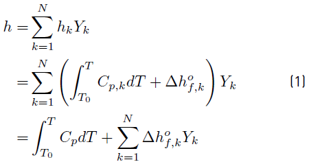
where C
p,k
is the mass heat capacity at constant pressure of species k, and
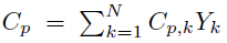 is the mass heat capacity at constant pressure of the mixture.
 is the formation enthalpy of species k, and
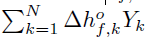 is the chemical enthalpy related to the whole reacting process.
The sensible energy e s,k (Equation (2)] and sensible enthalpy h s,k of any species k, are related by [34]
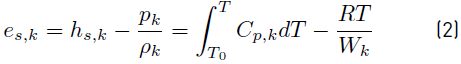
and then, the sensible + chemical energy e for the mixture of N reacting species becomes [34]
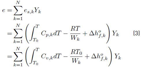
To obtain Equation (3), the relation between the mass heat capacities (Equation (4)] [34]
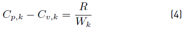
has also been used. Note that the R is the universal gas constant and W k the molecular weight of species.
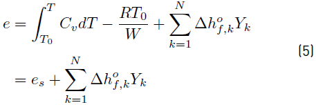
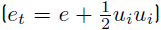
Finally, e (Equation (5) ) can be written as [34]
where C
v
=
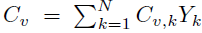 , and e
s
is the non-chemical sensible energy involving all the species.
, and e
s
is the non-chemical sensible energy involving all the species.
2.1 The total energy
Let’s consider first the conservation equation for total energy
 (Equation (6)], as it is given by Kuo [34]:
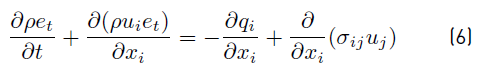
The heat flux q i (Equation (7) ) is written [34]
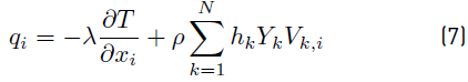
and includes, first a heat diffusion term expressed by Fourier’s law and a second term associated with different enthalpies which is specific to a gas with multi-species. Viscous and pressure tensors are combined into the σ
ij
tensor (σ
ij
= τ
ij
− p δ
ij
). External heat source terms due, for example, to an electric spark, a laser or radiation flux whose rates usually written
 , are not accounted. The power produced by volume forces f
k
on any species
, are not accounted. The power produced by volume forces f
k
on any species
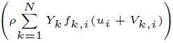 , is also not accounted.
The above expression for total energy (Equation (6)], is not always easy to implement in classical CFD codes because they use expressions for the energy, including chemical terms in addition to the sensible energy. Furthermore, the heat flux includes new transport terms. The use of only sensible energies (or enthalpies) are sometimes preferred [32,34].
2.2 The use of a total non-chemical energy
The sum of sensible and kinetic energies leads to a total non-chemical energy
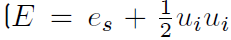 , Equation (8)], and the equation for E becomes [34]:
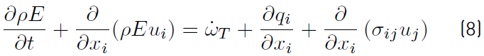
Where
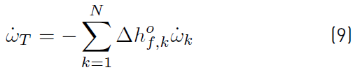
is the total rate of heat release due to chemical activity (Equation (9)] of all species. If the pressure p is added to ρE can be obtained Equation (10): [34]
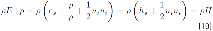
being H the non-chemical total enthalpy. The left term of Equation (8) can now be written [34]
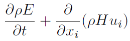
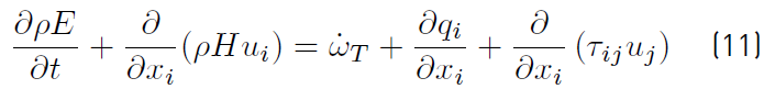
and the total energy equation for E (Equation (11)] that Will be used for now on is [34]:
2.3 Reynolds and Favre averages
The time-averaged equations are obtained by decomposing each flow variable into a mean and a fluctuating part. In constant density flows, Reynolds averages consist in splitting any quantity f into a mean f and a fluctuating f′ component
 . However, Reynolds averages in variable density flows introduce many other unclosed correlations between any quantity f and density fluctuations
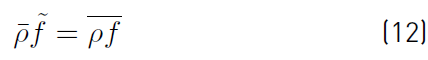
 . To avoid this difficulty, mass-weighted averages (Favre averages, Equation (12)] are preferred [32,34-37]:
Therefore, any quantity f splits into mean and fluctuating components as
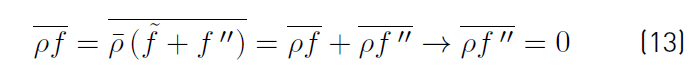
 . Note that time averages of double primed fluctuating quantities are not equal to zero. Instead, the time average of the double primed fluctuation multiplied by the density
 gives (Equation (13)]
 averages. Comparisons between numerical simulations providing Favre averages
 with experimental data, are not obvious. Most experimental techniques
provide Reynolds averages
 (for example, when averaging thermocouple data). Differences between (
) and (
) may be significant [32].
(for example, when averaging thermocouple data). Differences between (
) and (
) may be significant [32].
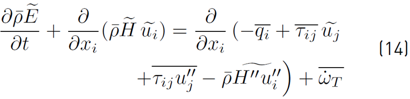
2.4 Favre’s averages applied to the total energy equation
Substituting the decomposed variables in Equation (12) and Equation (13) into the energy Equation (11) and averaging the results, the desired time averaged energy equation (Equation. (14)] can be written [32]:
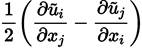
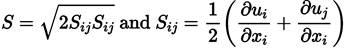
For a Newtonian fluid, the average stress tensor (τij , Equation (15)] is modeled as follows [38]:
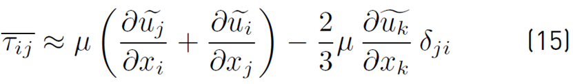
This approximation implies that the effects of turbulent fluctuations on the molecular viscosity (μ) are ignored, and the conventional
 and mass-weighted
 average velocities are approximately equal.
The term
 is well approximated (Equation (16)] for non-compressible flows by the following expression [38]
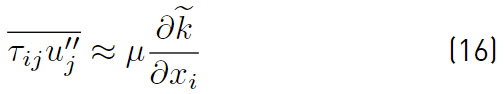
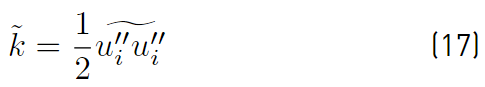
where
 is the turbulent kinetic energy (Equation (17)] [38]
For compressible flows, it can be assumed that this relationship remains valid.
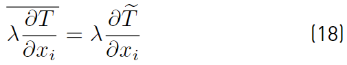
The time average heat flux vector
 contains contributions from heat conduction and an energy flux due to inter-species diffusion (Equation (7)]. If turbulent fluctuations effects are ignored when evaluating the thermal conductivity (λ), as it was done with the viscosity (µ), the contribution of heat conduction (Equation (18)] can be written [38]
The energy flux due to inter-species diffusion will be considered later and its treatment will depend on the model chosen for the species diffusion velocity. So, the term to be next modeled is
 .
.
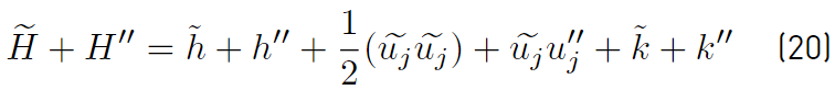
The average mass-weighted total enthalpy (Equation (19)] written regarding the static enthalpy h and kinetic energy terms, is [32].
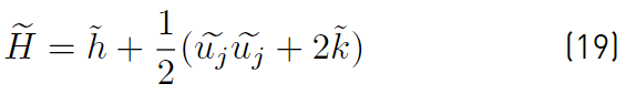
and from its instantaneous expansion it is obtained
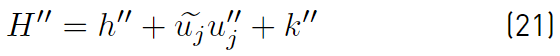
Now, subtracting Equation. (19) from Equation (20), only the fluctuating component of the total enthalpy (Equation (21)] remains, i.e.
The unclosed correlation
 given in Equation (14), can be expanded to yield [32].
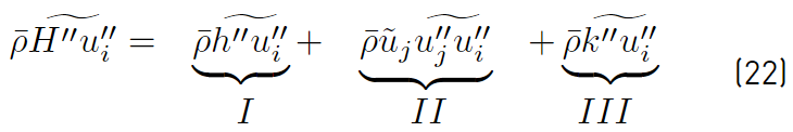
The first of the terms on the right side of Equation (22) is the Reynolds heat flux vector, which has historically been modeled using the gradient diffusion hypothesis (Equation (23)]. This model leads to the following expression for the Reynolds heat flux [32].
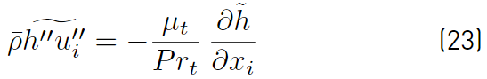
The turbulent Prandtl number (Pr t ), determines the ratio of the rate of turbulent momentum transport to rate of turbulent energy transport. Constant values for the Prandtl number are usually assumed, even though it has been shown to vary spatially [39].
The third term
 (Equation (24)] represents turbulent transport of the turbulent kinetic energy, and the gradient diffusion approximation is commonly used to model this term [32],
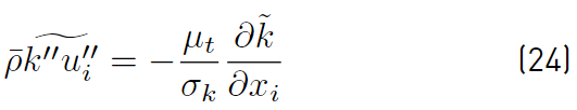
where µt is the eddy viscosity and σ k is a closure coefficient defined by the chosen model for turbulence.
The second term of the right side of Equation (22), is the dot product of the mean velocity with the Reynolds stress tensor. It is closed based on the model chosen for the Reynolds stress tensor. The most common closures used for the Reynolds stress tensor are linear models based on the Boussinesq approximation as shown in Equation (25) [32].
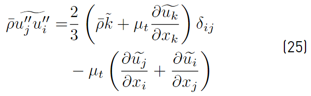
This model assumes that the Reynolds stress components are related to the mean strain rate tensor through an isotropic eddy viscosity (µ
t
). Models for the eddy viscosity vary from simple algebraic (zero equation) models [40], which require specification of a turbulent velocity and length scale, to two equations models [38,41,42]. In the two equations models, two partial differential equations are solved, one for the turbulent kinetic energy ( ), and other for the dissipation rate per unit mass
 or for an average turbulent dissipation rate
 . In the former approach, the
 model is achieved, and in the second one the
 .
.
Algebraic models are numerically robust and easy to implement (at least for simple geometries). However, they require changes in their coefficients when applied to different types of flow fields and ambiguity often arise when defining turbulence scales for complex geometries. Two-equation models have a more extensive range of applicability into complex geometries where it may be challenging to determine applicable turbulent scales algebraically. Nevertheless, one equation models that involve solving a transport equation for a quantity that can be directly related to the eddy viscosity [43,44] have gained popularity in recent years.
2.5 The RANS approach
For the RANS approach, closure models are based on a two-equation system that defines a transport equation for
 and an additional transport equation. This additional equation is based either on the average dissipation rate per unit mass
 or an average turbulence dissipation rate
 (
(
 or
or
 models). The shear stress transport (SST) models developed by Menter, the SST from 1994 [41] and the SST from 2003 [45] are adopted and here are presented.
Standard Menter SST Two-Equations model (SST-1994)
The Menter basic idea, is to keep the formulation of Wilcox’s
 [38,41,46] model applicable in inner parts of the boundary layer and all the way down to the wall, and take advantage of the Wilcox’s
model [38] in areas where it performs better (free streams flows, especially in the presence of adverse pressure gradients and in separating flows). To achieve its objective, Menter transforms the
[38,41,46] model applicable in inner parts of the boundary layer and all the way down to the wall, and take advantage of the Wilcox’s
model [38] in areas where it performs better (free streams flows, especially in the presence of adverse pressure gradients and in separating flows). To achieve its objective, Menter transforms the
 model into a variant of the Wilcox’s k−ω model, adding a term called cross-diffusion and also, changing the closing constants as the distance from the contour wall increases. The procedure followed by Menter to obtain his
− SST model is presented next [45].
model into a variant of the Wilcox’s k−ω model, adding a term called cross-diffusion and also, changing the closing constants as the distance from the contour wall increases. The procedure followed by Menter to obtain his
− SST model is presented next [45].
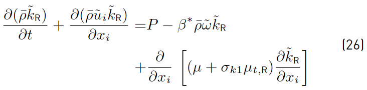
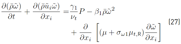
Wilcox k − ω original model (Equation (26) and Equation (27) ) [41]:
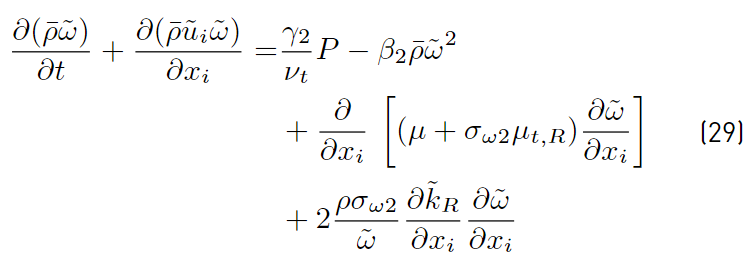
Menter proposed variation of the Wilcox’s k − ω original model (Equation (28) and Equation (29)] [41]:
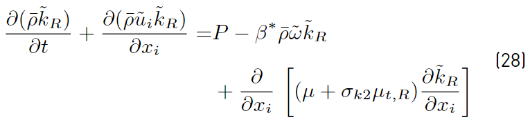
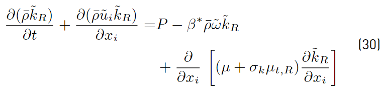
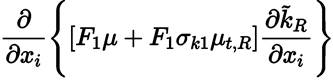
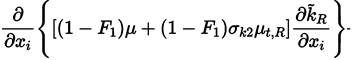
Multiplying each term of Equation. (26) by a sort of blending function F1(later to be defined), and each term of Equation (28) by (1 − F1) and after adding both, the equation for the energy kR of the turbulence is obtained [41]:
Proceeding in the same way with Equations (27) and (29), it can be obtained [41].
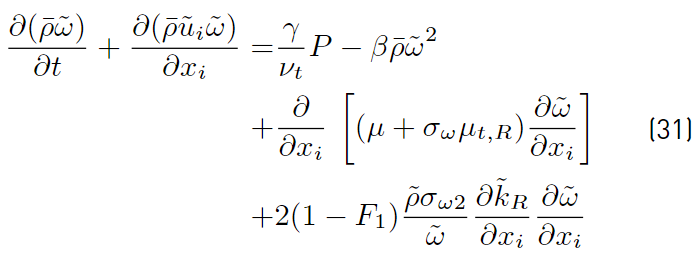
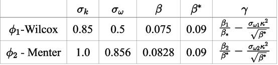
The last two equations (Equations (30) and (31)] are those of Menter model. The closing constant are obtained applying the relation given by Equations (32) [41].

being ϕ 1 and ϕ 2 given by Equation (33) [41]

An illustrative example of the use of Equation (32) for calculating the constants in Equations (30) and (31) is here included:
First, the last term of Equation (26) is multiplied by F1
Second, the last term of Equation (28) is multiplied by (1 − F1), obtaining
Adding the term coming from Equation (22) to the term coming from Equation (28), the result is [41].
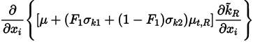
and finally applying the relation defining ϕ (Equation (32)], the above term reduces to
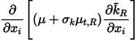
which is the way it is, shown in Equation (30).
Constants of the set ϕ 1 −Wilcox and of the set ϕ 2 −Menter, are presented in Table 1.
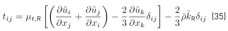
Additional functions needed to complete the Menter model are given by Equations (34), (36) and (37) [41].
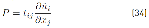
being t ij the turbulent stress tensor given by Equation (35) [46]
The function F1 [41,47], that it is used to couple the constants of the Wilcox and Menter models, is
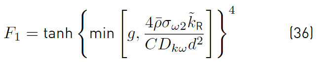
where
 is given by:
and CD kω by
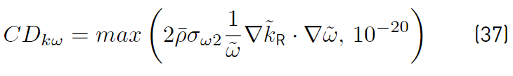
and d is the distance from the field point to the nearest wall, it should be noted that the function F1 has been designed so that its value is 1 in areas close to contour surfaces and 0 in distant areas.
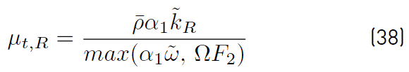
The turbulent eddy viscosity µ t,R (Equations (38)] is given as [41]
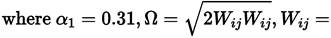
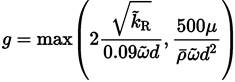
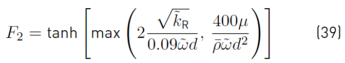
 and the function F2 (Equations (39)], is defined as [47]
Menter SST Two-Equations Model from 2003 (SST-2003)
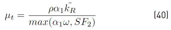
The SST Menter from 2003 has introduced several changes to the SST from 1994. The main one is the definition of the eddy viscosity (Equation (40)] which is now written [45]
Where
 . That is, in the definition of eddy viscosity, it is no longer used the magnitude of vorticity. The function P in both the
 and
and
 equations is replaced by min P, 10β
 , which implies the introduction of a limiter to P values. The definition of CD
kω
is changed by using in its second term 10−10, instead of 10−20. Finally, constants γ
1
and γ
2
are slightly different (the value γ
1
is ∼ 0.43% higher than the original one and the value γ
2
is lower by 0.08%).
, which implies the introduction of a limiter to P values. The definition of CD
kω
is changed by using in its second term 10−10, instead of 10−20. Finally, constants γ
1
and γ
2
are slightly different (the value γ
1
is ∼ 0.43% higher than the original one and the value γ
2
is lower by 0.08%).
2.6 The LES approach
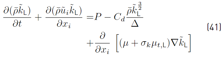
The closure problem in LES can be approached in a similar way as in RANS by defining an alternative to Equation (26). Following [48], one equation model is presented that defines the transport equation for
 as shown in Equation (41) (The subscript L stands for LES).
where t
ij
(the turbulent stress tensor, Equation (35)], is given substituting
 with
with
 and the eddy viscosity µ
t,R
(Equation (42)] with µ
t
,
LES
:
and the eddy viscosity µ
t,R
(Equation (42)] with µ
t
,
LES
:
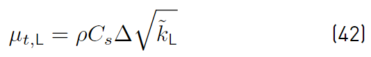
where ∆ is the characteristic length of cells. It implies the decomposition into different zones of the energy spectrum concerning a cutoff wave number k c , given by the grid size. Yoshizawa’s model assumes ∆ to be the cubic root of the cell volume. In Equations (41) and (42), C d and C s constants are related to the Smagorinsky constant C smag (Equation (43)] [49]
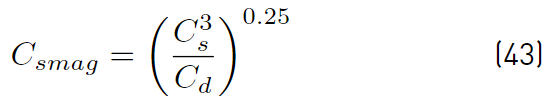
The Smagorinsky constant typically ranges from 0.065 to 0.2 and on any work, a constant value has to be assumed within the range given (Yoshizawa’s values for the constant C s and C d are 0.046 and 1.0 respectively). Furthermore, the value for σ k = 1.0.
2.7 The DES approach
The detached eddy simulation (DES) was developed as a hybrid approach to merge LES and RANS. The reason behind the development of DES is to attempt to reduce the number of points required for accurately solve the flow close to the wall in 3D simulations. To solve with LES the flow close to the wall, that is in less than 10% the size of the computational domain, over 90% of the grid points are needed [50]. To overcome this difficulty, the RANS approach is used close to the wall where it is known to provide accurate mean boundary layer predictions.
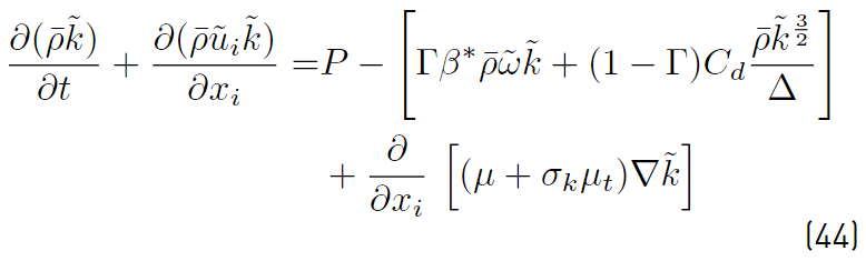
Equations (26) and 41, RANS and LES models, can be blended together (Equation (44)], resulting in the following
 transport equation [47]
The eddy viscosity µ t (Equation (45)] is obtained by blending the µ t,R and µ t,LES in the following manner

The blending function Γ (Equation (46)] is defined as
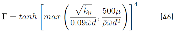
Depending on the value of Γ, there are three possible regions in the flow:
1. The RANS region, where Γ = 1. The closure is given by equations (30) and (31), and
 .
.
2. The LES region where Γ = 0. Equation (41) recovers and leads to
 .
.
3. An intermediate region where Γ is less than 1, but greater than 0. In this region, equation (44) applies.
Note that the
transport equation is solved everywhere in the computational domain to guarantee continuity, but it is not used in regions where LES is applicable.
2.8 The energy flux due to inter-species difusión
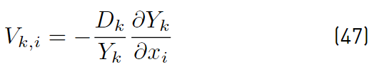
The diffusion velocity of any species k is usually evaluated from Fick’s law as shown in Equation (47) [32].
when the Reynolds averaged equation set is considered. It is usually accepted that the turbulent diffusion can also be expressed through Fick’s law. Further, it is also assumed that V i and D are the same for all species, assumption justified by the premise that an ”effective” turbulent diffusion dominates the molecular diffusion processes throughout most of the flow field. Then [32]
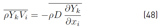
And
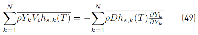
These two expressions (Equations (48) and (49)] simplify to the following (Equations (50) and (51)] [32]:
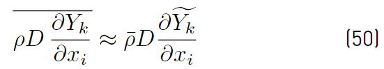
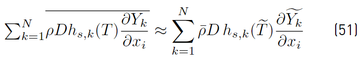
which implies that turbulent fluctuations effects are neglected on the mixture diffusivity, and conventional averages assumed equivalent to mass weighted averages. It is worth noting that the effect of temperature fluctuations on species enthalpy has to be ignored to arrive at the above expression for the averaged interspecies diffusion terms. The turbulent transport of a scalar property has always been modeled using the gradient diffusion approach. For instance, the Reynolds mass flux (Equations (52)] can be modeled as [32].
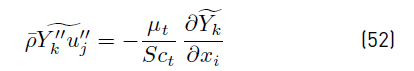
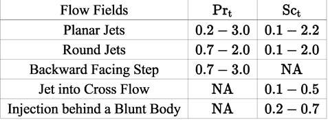
The turbulent Schmidt (Sct) number defines the ratio of the turbulent momentum transport rate to the turbulent mass transport rate. Constant values for the Schmidt number are usually assumed in applications of engineering interest, even though values for this coefficient have been shown to vary spatially [39].
The terms that generally require most attention by model developers are: the Reynolds stress tensor
 , Reynolds heat flux vector
 Reynolds mass Flow vector
 , and the chemical source term
 . The turbulent diffusion rates are controlled by turbulent Prandtl (Pr
t
) and Schmidt (Sc
t
) numbers. Constant values for these numbers are usually assumed in applications (in low as well as in high speed reacting flows of engineering interest), even though values for these coefficients have been shown to vary spatially [Table 2, [39])
. The turbulent diffusion rates are controlled by turbulent Prandtl (Pr
t
) and Schmidt (Sc
t
) numbers. Constant values for these numbers are usually assumed in applications (in low as well as in high speed reacting flows of engineering interest), even though values for these coefficients have been shown to vary spatially [Table 2, [39])
Numerical studies have suggested that when attempting to characterize high-speed devices (that contain a variety of different mechanisms) with constant turbulent transport coefficients, care is required.
3. Chemical production rates
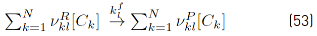
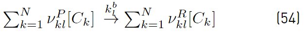
The most common species production rates used for reacting flows are built based on a laminar chemistry formulation. This approach based on laminar chemistry assumption ignores turbulence-chemistry interactions by evaluating the chemical source terms based only on mean flow properties. Any of the reactions between the N species, can be written in a compact form as shown in Equations (53) and (54) [51].
where
 and
and
 are the reactant and producto stoichiometric coefficients for species k,
 and
and
 the forward and backward rate constants of any reaction l from the total number of reactions nR. [C
k
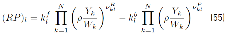
] is the molar concentration of species k involved. After introducing the mass reaction rates (ρY
k
/W
k
), being W
k
the molecular weight of the species, the rate progress (RP)
l
(Equation (55)] of reaction l can now be written as follows [34]:
the forward and backward rate constants of any reaction l from the total number of reactions nR. [C
k
] is the molar concentration of species k involved. After introducing the mass reaction rates (ρY
k
/W
k
), being W
k
the molecular weight of the species, the rate progress (RP)
l
(Equation (55)] of reaction l can now be written as follows [34]:
If forward rates and the equilibrium constants are used to determine backward rates [32,34], the rate production of species k due to reaction l, is written in the form shown in Equation (56)

Note that on the rate production
 for species k, the factor α
l
accounts for third body effects. Finally, the total rate of species k is the nR sum of rates
(Equation (57)] produced by each reaction, therefore [34].
for species k, the factor α
l
accounts for third body effects. Finally, the total rate of species k is the nR sum of rates
(Equation (57)] produced by each reaction, therefore [34].
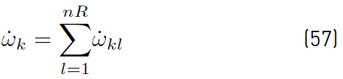
This value
 is used when the heat released
 , due to chemical activity of all the species is computed (Equation (9) ). The matrix of stoichiometric coefficients resulting from any chemical system has dimension N × nR, and from this matrix, a set of N stiff ODES in each control volumen and time step, must be assembled and solved [52].
4. The model for the equation of state
It is assumed that the fluid behaves as a mixture of perfect gas (Equation (58) ). Therefore the pressure p is given by [32]
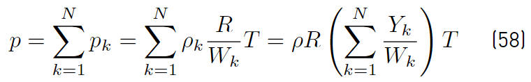
Since the mixture gas constant (Equations (59)] is defined by [34]
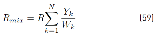
the equation of state (Equations (60) ) can now be written as [34]
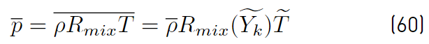
where to minimize closure difficulties, the effects of composition fluctuations on the equation of state are neglected.
5. Conclusions
In this paper, essential aspects of RANS, LES, and DES methodologies for turbulence modeling are described. The needed theoretical formalism to develop and closure an energy equation applicable to turbulent reactive flows was discussed. This work was motivated because the authors consider that models built based on theoretical arguments are more satisfactory than models built from practical arguments, even if a practical model provides better results for one specific case. However, in industrial as well as in academic environments, the available computational framework has a strong influence when decisions are to be made.

