Identifying a greenhouse climate model by using subspace methods

Fredy Orlando Ruiz Palacios¹ y Carlos Eduardo Cotrino Badillo²

¹ Electronic Engineering, Pontificia Universidad Javeriana (PUJ), Bogotà, Colombia. M. Sc., Universidad Javeriana (PUJ), Bogotá, Colombia. Ph.D., Research, Politecnico di Torino, Italia. Assistant Professor, Pontificia Universidad Javeriana (PUJ), Bogotá, Colombia. ruizf@javeriana.edu.co ² Electronic Engineering, Pontificia Universidad Javeriana, Bogotá, Colombia. M Sc, SUNY at Stony Brook. Associate Professor, Pontificia Universidad Javeriana(PUJ), Bogotá, Colombia. ccotrino@javeriana.edu.co

Abstract

This paper presents the development of a climate dynamics model for a greenhouse located on the Bogota plateau. A black-box model was estimated from experimental data, considering a novel system structure derived from a first principles model and experimental tests. It considered two control volumes, one given by the air over the crop and a second one formed by the air trapped by crop foliage. The model was selected from a set of linear, discrete-time, state-variable systems using subspace identification methods. The estimated system was able to predict climate dynamics for both control volumes, having errors below 8%. Such performance was comparable to previous work reported in literature while the obtained model was a low-complexity linear system.

Keywords: Parametric estimation, subspace identification, greenhouse climate model.

Received: november 24th 2009

Accepted: may 11th 2010

Introduction

Even though agriculture is a millenary old economic activity, using tools like automatic control and model identification have only been introduced during the last few decades. Instrumentation and control strategies have been developed and applied for optimising crop production since the 1960s and, more recently, modern modelling and identification tools have enhanced the forecasting and prediction of the climate variables inside a greenhouse environment. Most of these models and applications come from Europe where the summer and winter seasons' extreme temperature make the rational use and optimal control of HVAC equipment required to protect the plants mandatory in such extreme conditions. G.P. Bot at Wageningen Agricultural University has developed dynamic models for greenhouses in the Netherlands and Indonesia from biological basic principles (Bot 1983). Further work includes external weather conditions for designing energy control systems (Körner 2003, Tap et al., 1996, Bot 2001). P.F. Martínez at the Universidad Politécnica in Valencia has applied genetic algorithms to building a non-linear green house model for Mediterranean conditions (Herrero et al., 2003).

J.B. Cunha at the Universidade de Tras-Os-Montes e Alto Douro has used recursive identification techniques for building several climate models, comparing their results and configuring different control strategies for optimising energy consumption (Cunha 2003), (Cunha et al., 1997), (Cunha et al., 2003).

Ghoumari (Ghoumari 2003) built a non-linear model predictive controller with restrictions; the climate model was obtained from basic principles and calibrated by sequential quadratic programming.

Peter Young at Lancaster University has developed statistical methods for identification and control and applied them to automatic control of greenhouses in Bedford, UK (Young et al., 1994, Young et al. 2001).

This paper describes a new methodology for building a dynamic model of a greenhouse climate. The selected model was estimated from a set of linear, time invariant models, using experimental data. The results of this procedure, weighted as being the error between measured variables and predicted ones, showed that a low complexity, third-order linear model described internal climate dynamics with a precision close to that of more complex first principle-based non-linear models.

Experimental configuration

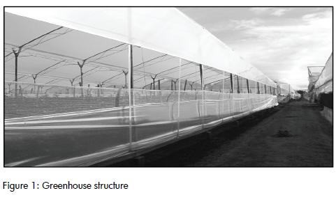
The modelled greenhouse was located in the country side of "El Rosal", a small village on the Bogota plateau lying at 2,586 meters above sea-level, having an annual average temperature of 14oC. It covered an area of 6,314 m² (77 m x 82m) and had variable height of 2.9 m for the lateral walls and 4.3 m in the central part, giving 23,000 m³ total volume. Side ventilation was manually controlled and zenith was fixed, covering 370 m², close to 5.6% of total area (Figure 1). The covering material was average transparency polyethylene. There were no manipulated variables and the model reflected the effect of external weather conditions on internal greenhouse climate variables.

Temperature and relative humidity (RH) were measured and logged with a WatchDog 450 (Spectrum Technologies) having ± 0.6°C and ± 3% RH accuracy. PAR radiation, from 400 to 700 nm, was measured with a PAR Quantum sensor (Spectrum Technologies). These measurements were transformed to total energy (W/m²) over the full solar radiation spectrum, this being a valid calculation since the solar radiation spectrum is very well-defined, as reported by Wang et al., 2000, and Kania et al., 2002.

Temperature and RH were registered at 8 different sites inside the greenhouse: 4 of them placed at 2.5 m above ground level and at symmetric locations and the other four were located inside crop foliage at 1.2 m above ground level and in the same ground bed. Side ventilation inlets were kept at 50% opening throughout all the experiments, this being the greenhouse's normal operating point. Figure 1: Greenhouse structure A temperature and RH recorder was installed far away from the greenhouse structures to ascertain external weather variables so that any influence from the greenhouse environment was negligible. This recorder was placed at 1.5 m above ground level.

Sampling time was fixed at 5 minutes for all experiments and variables, based on instrument response time, logger memory size and the time settings reported by other authors (Körner et al., 2004), (Cunha et al., 1997), (Salgado et al., 2005), (Wang et al., 2000).

The row data from the meters had to be conditioned and set in the format required by the software tool for identification, as follows:

– RH was converted to absolute humidity, χ, this transformation uncoupled the humidity measurement from temperature and allowed using the mass conservation equation for water regarding χ, instead of RH, which is a non-linear function of temperature and absolute humidity.

The transformation was defined by the equation:

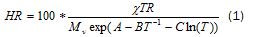
T T temperature (K); R universal gas constant, water molecular weight and constants A, B and C.

–The four temperatures and RH measurements of greenhouse air were averaged to obtain lumped parameter approximation.

–Since a PAR measurement was available and there was no artificial illumination, all the incident radiation was coming from the sun. PAR data (Q_par ), was converted to radiated power over the complete spectrum ( Q_rad). The conversion was done using the relationship:

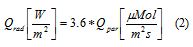
3.6 was a scale factor having the proper units (Kania et al., 2002).

Model selection

This section describes a lumped parameters model along with the model structure used for identifying the greenhouse climate.

Theoretical model

A model for the greenhouse's internal climate was built from energy and mass conservation laws. Strictly, climate evolution at every point of greenhouse volume would be different and the resultant model would, therefore, be a distributed parameters one, described by a set of partial differential equations having boundary conditions at each interface with the external environment (Molina-Aiz, F 2004). This type of model would be highly complex, having infinite dimensions and useless for drawing analytical conclusions and for designing a control system.

Assuming uniform temperature, T_a , in the control volume limited by the air enclosed in the greenhouse, the energy conservation equation would be:

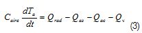(3)

Where: C_aire was greenhouse air thermal capacitance and Q_rad the heat flow coming from solar radiation. Q _as was heat flow due to the temperature gradient between air and soil. Q_ac was heat flow through the plastic cover due to the temperature difference between internal and external air and Q_v was the heat flow associated with air exchange through greenhouse ventilation openings.

A second control volume was defined to enclose a layer of soil interacting between greenhouse air and sub soil (Bot 1983). The equation for soil temperature T_s was:

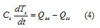
C_s was soil thermal capacitance and Q_ss heat flow due to the temperature gradient between the soil and the sub soil. This approach considered that sub soil temperature was an input variable, not manipulable and independent of greenhouse climate.

Absolute humidity χ, was the amount of water vapour present in the air, measured as the mass of water vapour per volume unit. Its behaviour inside a limited volume was described from a mass balance in the control volume (Tap 1996)

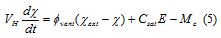
V_h greenhouse effective volume;Ø_vent(χ_ext −χ) net water vapour flow in or out bound the control volume; E was crop transpiration produced by biological phenomena, C_sac water in air saturation constant and M_c was the vapour condensation on the greenhouse walls and on crop leaves.

These three equations (3), (4) and (5) were non coupled differential equations and corresponded to the greenhouse climate model's state variable formulation.

The hardest step, when formulating a theoretical model for a specific greenhouse, stems from the complexity estimating each

equation term, since all heat and vapour flows are non-linear functions of both internal and external climate conditions, and, all equations parameters depended on greenhouse layout, dimensions, type of plant grown and other biological factors.

Parametric model

A linear, discrete, time-invariant model was estimated to describe the greenhouse climate from the experimental data gathered from the field-work. The model was assembled as a multiple input, multiple output dynamic system using state space formulation. This model was identified by using available algorithms which are efficient and robust.

The resulting model consisted of a set of first-order difference equations:

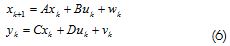
Where k was the independent time variable; u_k∈R^m was a vector of m process inputs at instant k, y_k∈Rⁱ was a vector of l process outputs at instant k,; x^k∈Rⁿ was a vector of n process state variables at instant k,w _k ∈ Rⁿ and v^k∈ Rⁱ were vector arrays of stochastic, non-measurable variables presenting noise in the process and in the measurements. These variables were assumed to be stationary white noise having zero mean, related by:

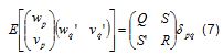
Matrices A,B,C,D described the state space model. were the covariance matrices for the noise sequences. These seven matrices had to be estimated from the experimental data gathered during the experiments and conditioned, as already described.

Selecting the variables

Even though several authors have assumed that the greenhouse environment is uniform in a vertical direction (Piñon et al., 2002, Trigui et al., 2001, Herrero et al., 2003, Bot 1983), the experimental data for this greenhouse showed a significant gradient between the air close to the plants and the air over the plants.

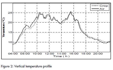
Figure 2 illustrates temperature variations in a vertical direction at any point inside the greenhouse. Air temperature close to the foliage showed a time delay for heating and cooling cycles. Furthermore, the rap id temperature changes experienced by the upper air were attenuated by the foliage. These two facts were represented in the model by a low pass filter, which increased model order.

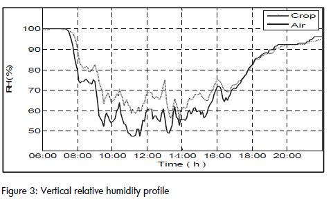
Evapotranspiration is the flow of water vapour from the plant towards the air. Several empirical models have described this phenomenon; flow is a function of the solar radiation captured by the plant, leaf temperature and vapour pressure deficit in all of them, accounting for the difference between current partial vapour pressure and vapour saturation pressure. When this deficit was close to zero, leaves did not release vapour and net flow to the environment was zero. As shown in (Figure 3), this behaviour agreed with the experimental data.

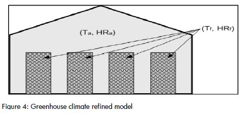
Even though the vertical gradients were significant, it was still possible to develop a lumped parameters model by defining two control volumes (Figure 4). The first one enclosed the air in the greenhouse volume outside the foliage and corresponded to the “internal air volume” used in most models. The second volume corresponded to air entrapped inside the foliage. There was heat exchange in the interface between the two regions due to conduction and convection and mass flows produced by differences in partial pressure. The structure of the model to be identified was:

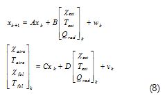
The input variables were: χ_ext the external air absolute humidity; T_ext external air temperature and Q_rad solar radiation. The output variables were: temperature T_aire and absolute humidity χ_lof of greenhouse internal air and temperature T_fol and absolute humidity χ_lof of the foliage trapped air.

Since the micro climate of foliage entrapped air was heavily dependent on the type of crop and plant distribution and concentration, all the temperature and RH data measured were used directly in the identification procedure. These approximations were supported by the unidirectional nature of the relationship between both volumes. The climate of the air over the crop affected the climate of foliage entrapped air but this was not true in the reverse direction, since the volume of free air was much larger than the volume of entrapped air.

Experimental results

Two sets of measurements were gathered over different days for identifying the process model described by equation 8. The first, named "identification set," included 1,650 samples of each variable, taken over a period of 138 hours. This set was used for estimating model order n and matrices A, B, C and D. The second set, named "validation set," included 860 samples taken over a period of 72 hours. This data was used to test the quality of the resulting model, evaluating the identified model's predictive capabilities with a data set not used for model construction.

Model order estimation

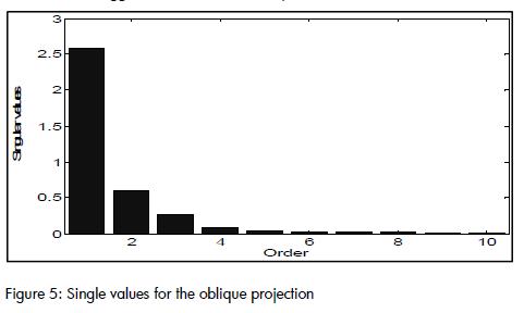
The method used for building the model was the sub space identification method developed by Overchee et al., 1996. In this approach, model order corresponds to the number of non-zero singular values of the oblique projection of the subspace spanned by those future output variables parallel to the future input variables space, over the space spanned by the past inputs and output variables. Intuitively, the dimension of the projected subspace corresponds to the content of future outputs which cannot be generated by future inputs and, therefore, must be generated by the system's past history. The singular values of the oblique projection for the identification data set are shown in Figure 5 From these results, the suggested order for the system was n=3.

The physical model described in the previous section and the field experiments suggested a model order n = 3. One differential equation described the behaviour of the air over the plants and another one the foliage entrapped air temperature, related to air temperature through a low pass filter. No equation was required for entrapped air humidity since its dynamic were close to that of over air humidity, having a variable bias function of temperature, vapour pressure deficit and solar radiation.

Model response

Using the Overchee et al., 1996 identification algorithm via subspaces combining deterministic and stochastic variables, model order was n = 3. A percentage simulation error was applied to assess the quality of the resulting model:

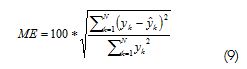
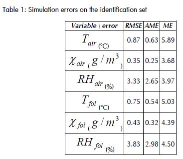
Where: Y_k was output variable estimated by the model; measured output variable and N samples number or experiment time length. Table 1 summarises identified model outcomes on the identification set. Additional to ME error, two other measurements were included: root mean squared error (RMSE) and absolute mean error (AME).

The ME was less than 6% for all estimated variables. Humidity was predicted with ME 2 percentage points lower than temperature.

The second quality test for the identified model was a simulation of the greenhouse climate using validation set data. Resulting errors are listed in Table 2.

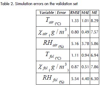
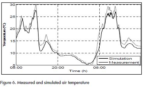
The identified model closely described the evolution of air and foliage temperatures. RMS error was 1.33°C, but instrument precision was 0.6°C. Figure 6 shows the variation of air temperature using validation set data. The model closely followed the temperature variations, except for the higher values where the model predicted somehow lower temperatures than the actual ones.

For the air relative humidity, the model produced convenient data for daylight periods, when RH was low (Figure 7). At night, when there was saturation of water vapour in air, model outcomes did not match the actual data. This was due to the non-linear characteristic of this process: plant evapotranspiration stoppede and a negative flow showed up due to water condensation on the plastic side walls and on plant leaves. The linear model failed to describe this behaviour and, at some intervals, RH rose to over 100%.

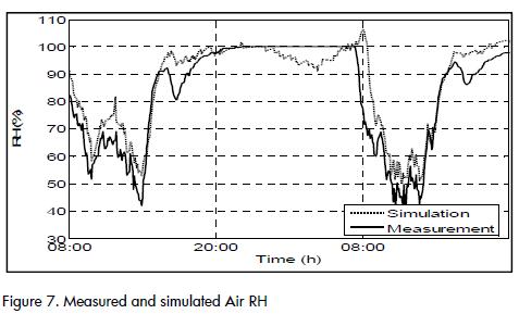
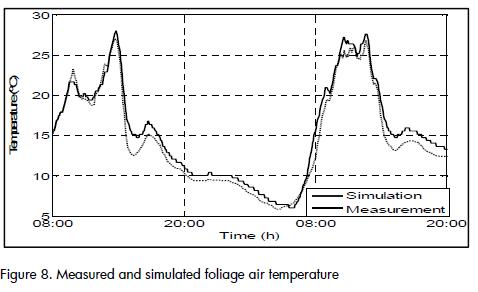
Figure 8 shows convenient correspondence between measured and estimated data for temperature for the variables in the air entrapped in the foliage.

Identified model performance was comparable to models reported by other authors (Wang et al., 2000), (Cunha, 2003), (Herrero et al., 2003) and (Salgado and Cunha, 2005) where RMSE errors were around identified model results within reported error ranges: RMSE values around 1.5°C for T_aire and 5% for χ_aire . The proposed model showed some additional features; it was a low order lineal model and it adequately described the climate inside the foliage.

Conclusions

The paper has described the development of a climate model for a greenhouse located in an inter-tropical region. The resulting model bore similar errors to those of equivalent order models reported in the technical literature using a linear structure. Even though the approach used did not rest on basic physical principles, knowledge and understanding of these principles is a key step in identification, since they allow comprehending the model structure and dynamic relationships and facilitate interpreting the resultant data and comparing it to actual measured data.

A second topic regarding identification was the selection of a possible model set, like state space representation choice and using an algorithm based on subspaces. Such selection was adequate for finding the multivariable dynamic system's parameters.

The modification introduced into the model's structure separating the dynamics of air volume over the crop from the dynamics of foliage entrapped air rendered better model quality without significantly increasing computational load. This structure has not been reported up to now and thus represents a novel contribution in this field of modelling.

More variables must be included in experimental and identification tasks for future work and to increase model quality. These variables would be wind speed and direction, soil and sub soil humidity and temperature.

A following step towards precision agriculture is the deployment of identified models for designing model-based control strategies aimed at production optimisation in climate-controlled greenhouses.