




 English (pdf)
 Article in xml format
 Article references

 Automatic translation
 Send this article by e-mail
 Cited by SciELO
 Cited by Google
 Similars in
SciELO
 Similars in Google

 Permalink


1. Introduction
The growing use of renewable technologies is illustrated in Latin America by the generation of 210 GW of low-carbon energy through hydropower, biomass, solar, wind, and geothermal [1]. The latter provides baseload energy with a lower environmental impact compared to other power generation methods [2,3].
To improve the sustainable use of geothermal resources, numerical simulations can be used to update conceptual models and to understand and predict heat transfer and fluid flow in geothermal reservoirs [4-7]. Here, faults can also directly affect geothermal fluid circulation. Their impact has been studied with experimental investigations [8], structural and kinematic data [9], and numerical modeling [10,11].
This paper presents the results of field characterization and numerical simulations of fluid flow and heat transfer in the geothermal system associated with the Nevado del Ruiz Volcano (NRV) in Colombia. The numerical simulator HydroGeoSphere (HGS) [12] uses the Discrete Fractured Models approach to represent regional faults embedded in a low-permeability porous rock matrix. The geothermal fluid is assumed to be in its liquid phase, before it flashes. [13] and [11] have simulated 2D heat transfer at the reservoir scale in the NRV with the numerical simulator OpenGeoSys In contrast, this work focuses on a specific zone located at the intersection of three faults (Samaná Sur, Santa Rosa, and El Billar) that defines an area of special interest for geothermal development and presents a 3D model. The influence of these faults on the local fluid circulation and a hypothetical geothermal production scenario are analyzed here, and they have not been presented before.
2. Geological setting
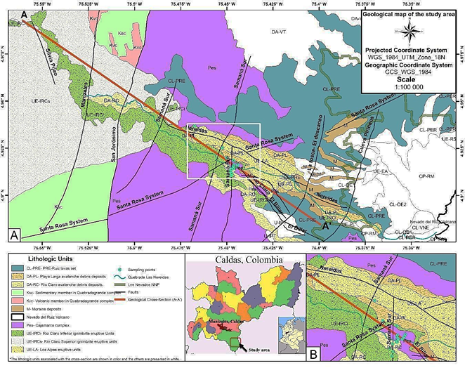
The study area is located to the West of the NRV complex, in the Nereidas sector. The geological units in thiszone area: the Cajamarca Complex (Pes), the Quebradagrande Complex (Ksc and Kvc), and the Quaternary eruptive and superficial deposits (Fig. 1).
Source: the authors, modified from [15] and [16].
Figure 1 Geological map of the study area, with cross-section AA’ (red line). The close-up in B shows the intersection among the Samaná Sur fault system with the Santa Rosa and El Billar faults.
The Cajamarca Complex comprises metamorphic rocks forming the nucleus of the Colombian Central Mountain Range [14]. It contains pelitic mica and quartz-sericite schists (Pes in Fig. 1), formed through regional metamorphic events and local thermal or dynamic effects of varying intensity.
The Quebradagrande complex is found between the San Jerónimo and Silvia Pijao faults (Fig. 1). It is an interrelation of volcanic (volcanic flows and pyroclastic layers) and sedimentary rocks [15]. The volcanic member (Kvc) consists of basalts and diabases with toleitic characteristics, some debris flow breccias, and tuff. The sedimentary member (Ksc) is predominantly recognized as carbonaceous lutite, graywacke, feldspathic arenite, limolithes, lidites, and local limestone layers [15].
The quaternary eruptive and superficial deposits are the result of the interaction and evolution of the volcanic processes that have marked the history of the zone. The PRE-Ruiz lavas (CL-PRE) form a homogeneous, dense, and eroded unit with the presence of bands that vary from light gray to white. The Río Claro Ignimbrite Eruptive Unit (UE-IRC) is divided into the Inferior Deposit Unit (UE-IRCi), which is massive, partially altered, poorly selected, and matrix supported. The Superior Deposit Unit (UE-IRCs) is massive, well sorted, crumbly, with medium to fine grain sizes, and very altered. The other deposits are the Playa Larga avalanche debris deposits (DA-PL), Los Alpes eruptive units (UE-LA), Río Claro avalanche debris deposits (DA-RC), and Moraine deposits (M) [16].
Structural geology is an important aspect for the study area since it contains several faults that generate both upward groundwater flow (evidenced by the presence of superficial hot springs) and downward groundwater flow (allowing reservoir recharge) [17]. The Silvia Pijao fault belongs to the Romeral fault system and is classified as a regional tectonic feature with N-S to NNE orientation and dextral reverse behavior [18]. [19] defined the Manizales-Aranzazu fault, called here the Manizales fault, with dextral reverse behavior. [16] defined the San Jeronimo fault with sinistral reverse behavior and NNE-SSW tendency. Moving towards the East, the Samaná Sur fault system (hereafter simply referred to as fault) is described with sinistral normal behavior and N-S to N20E orientation. Then, the Nereidas Fault presents a sinistral movement with normal behavior [16] with a dip between 50 to 60° NE [20]. The Santa Rosa Fault is defined by [21] with reverse dextral behavior, while the El Billar fault has sinistral normal behavior and a dip of S70W approximately. The Quebrada Negra fault presents normal behavior and a N20-40W dip [16]. Finally, the La Tosca- El Descanso is the easternmost fault crossing the AA’ trace (Fig. 1) and it is catalogued as the most recent in the study area, with a dextral behavior [20].
3. Field characterization
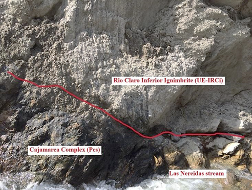
In the Botero Londoño area (4.915°N 75.45°W, WGS_1984_UTM_Zone_18N), the outcrop of the Cajamarca complex (Pes) underlying the Río Claro Inferior ignimbrite eruptive unit (UE-IRCi) was identified, in a valley containing several hot spring manifestations along Las Nereidas stream (Fig. 2). The schists of Pes (Fig. 3) have foliated nature, and their discontinuities (joints, random fractures, and faults) allow a fast circulation of hydrothermal fluids [20].
Source: The authors.
Figure 2 Lithological contact between the Cajamarca complex (Pes) and the Río Claro Inferior ignimbrite (UE-IRCi) identified in the field.

4. Hydrogeological numerical model
Cross-section A-A’ shows the main geological units in the study area, as well as the faults and geological contacts (Fig. 4). Its actual orientation is northwest - southeast (Fig. 1). A small correction should be applied to the orientation of the faults, but it is neglected here considering the uncertainty that still exists about their orientation and their continuity at depth [11].

Source: The authors.
Figure 4 Geological cross-section A-A’. The lithologic units shown here are grouped into the three hydrogeological units listed in Table 1.
Considering the hydraulic properties and spatial extension, three hydrogeological units are defined, and they are listed in Table 1) the Quebradagrande complex (Kvc and Ksc) that may act as an aquitard, 2) the Cajamarca complex (Pes), an aquitard that locally acts as a fractured aquifer hosting the geothermal reservoir, where the rock is highly fractured close to the faults, and 3) the superficial deposits that combine all quaternary units with limited thickness. The properties of each hydrogeological unit required for the numerical simulations are listed in Table 1.
Table 1 Properties of the three hydrogeological units defined in the model (data from 11, 13, 22).
| Properties | Pes | Kvc & Ksc | Superficial deposits |
|---|---|---|---|
| Hydraulic conductivity (m s-1) | 8.4x10⁻¹¹ | 9.8x10⁻¹¹ | 2.0x10⁻¹⁰ |
| Specific storage (m-1) | 1x10⁻⁴ | 1x10⁻⁴ | 1x10⁻⁴ |
| Porosity | 1x10⁻² | 0.1 | 0.1 |
| Longitudinal dispersivity (m) | 100 | 100 | 100 |
| Transversal and vertical dispersivity (m) | 10 | 10 | 10 |
| Tortuosity | 0.25 | 0.25 | 0.25 |
| Thermal conductivity of solids (W m-1 K-1) | 4.94 | 1.92 | 1.22 |
| Bulk density (kg m-3) | 2697 | 2654 | 2660 |
| Specific heat capacity of solids (J kg-1 K-1) | 910 | 822 | 815 |
Source: The authors.
Faults are modeled as 2D planes, where groundwater velocity is defined from Darcy’s law and the fault hydraulic conductivity is calculated according to the parallel plate conceptual model:

where 2b (m) is the fracture aperture, γ (N m-3) and μ (Pa s) are the specific gravity and the dynamic viscosity of water, respectively.
4.1. 2D model
The 2D numerical model (Fig. 5) is based on the geological cross-section (Fig. 4). The mesh is generated with AlgoMesh [23] using 5409 nodes and 10194 triangular elements, whose maximum and minimum areas were 146842 m2 and 4 m2, respectively. The mesh is refined close to the ground surface and near faults, to properly capture their geometry. Since HGS always uses 3D elements to discretize the subsurface, the 2D mesh is duplicated in the direction perpendicular to the cross-section to form 3D triangular prisms (6-node elements). Therefore, the resulting 3D mesh has a unit thickness in the direction perpendicular to the cross-section.

For groundwater flow, the upper and lateral boundaries are assigned hydraulic head values equal to ground surface elevation and the bottom is considered impermeable. For heat transfer simulations, adiabatic conditions are set to the left and right boundaries, while a constant average surface temperature of 15°C is assigned to the top. A spatially variable initial temperature distribution is applied to the model. The values were calculated with the local heat flux and thermal conductivities of the Pes and Kvc-Ksc formations shown in Table 1. A spatially variable heat flux is applied to the bottom of the model to represent the heat released by the magmatic chamber of the NRV. Two different heat flux values are assigned, according to the thermal properties of the Quebradagrande (Kvc and Ksc) and Cajamarca (Pes) complexes. The Kvc and Ksc complexes are assigned a heat flux equal to 0.12 W m-2, which is the smallest value according to the Colombian heat flux map of the region [24]. The assigned heat flux for the Pes complex is 0.6 W m-2 and it was calculated with Fourier’s law and the geothermal gradient of about 140°C/km reported for the Nereidas well [25]. For transient heat transfer, the total simulated time is 10 million years, while groundwater flow is simulated in steady-state conditions.
For modeling purposes, all superficial deposits are considered as a single hydrogeological unit with average hydraulic and thermal properties (Table 1) since their thickness is not significant when compared to the model dimensions. Finally, all faults are represented as discrete fractures, represented as two-dimensional planes with uniform apertures. Since the faults are poorly characterized because of difficult access in this remote area, a sensitivity analysis of fault aperture is conducted using values equal to 1x10⁻¹ m (Case A), 1x10⁻³ m (Case B), and 1x10⁻⁵ m (Case C), as listed in Table 2. The value of 1 mm (Case B) represents a base case, and the other two values are defined by increasing and decreasing the base case value by two orders of magnitude, to generate a significant difference between the three scenarios. The main purpose of the sensitivity analysis is to assess the impact of the fault apertures on groundwater velocity. These scenarios also show how the fluid mass balance changes depending on fault aperture.
4.2. 3D model
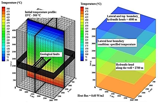
The 3D numerical model represents a hypothetical geothermal production vertical well that would intersect the Samaná Sur, Santa Rosa, and El Billar faults shown in Fig. 5B. The objective is to simulate hydraulic head and temperature variations that might result from 30 years of geothermal production. The model dimensions are 3000 m, 3000 m and 4000 m in x, y, and z directions, respectively (Fig. 6). The production well is located in the center of the domain, at x = 1500 m and y = 1500 m. It is open and connected to the subsurface between elevations 1400 m and 1800 m to represent the location of the well screen in the production zone. The depth of the model is defined considering the average temperature simulated in previous studies conducted in areas close to Botero-Londoño. According to results presented by [11] and [13], two kilometers would be an appropriate depth for electric generation since the simulated temperature in this zone is above 150 °C. A total depth of 4 km is thus considered here to keep the bottom of the well far enough from the model boundary. Similarly, in the x and y directions, it is assumed that the boundaries are far enough from the well.
Two porous medium zones are defined: the reservoir zone (Cajamarca complex) extends from the bottom up to an elevation of 2500 m and it is overlain by the caprock, which consists of eruptive and superficial deposits and extends to the top of the model at an elevation of 4000 m. The hydraulic and thermal properties are listed in Table 1.
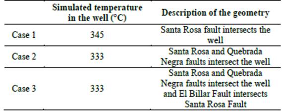
The depth of the three faults (Samaná Sur, Santa Rosa, and El Billar) is unknown. To analyze the impact of the intersection of faults with the production well on the cone of depression generated during withdrawal, three scenarios are defined. In Case 1, the production well only intersects the Santa Rosa fault, in Case 2 it intersects both Santa Rosa and El Billar faults, and, finally, in Case 3, the Santa Rosa and El Billar faults are intersected by the well, and there is an intersection between Samaná Sur and Santa Rosa faults. All three faults have the same aperture of 1 mm.
The mesh is generated by HGS, and it consists of 343914 nodes and 327936 block elements, which are refined near the faults and the pumping well. The internal diagonals or the sides of the 3D blocks are automatically selected by the HGS 2D fracture generation algorithm. Those 2D elements are selected using the three points that identify the fracture plane that must be entered by the user. Later, fracture properties are assigned to those 2D elements. Therefore, the resulting faults are represented by a staircase profile in the mesh (Fig. 9) and their angle with the well axis depends on the size of the block elements crossing the faults. A specific head of 4000 m is applied to the lateral and upper boundaries, while the bottom is assumed impermeable. Along the well screen located in the production zone, a hydraulic head of 2700 m is assigned to represent the pressure drawdown due to fluid flow through the reservoir, when production starts. The node at the top of the well has the same hydraulic head of 4000 m preventing the fluid above the well from migrating towards it, due to its high permeability. For heat transfer, an average temperature of 15°C is applied to the top, as done in the 2D model, while the bottom heat flux is 0.6 W m-2, which corresponds to the flux for the Cajamarca complex that forms the rock basement in the Botero-Londoño area. The lateral heat boundaries are assigned to a temperature that decreases from the bottom to the top of the model along four different zones with a thickness of 1000 m. The temperature for each zone is calculated from the average heat flux (0.6 W m-2). The temperatures assigned are, from bottom to top, 435°C, 345°C, 240°C, and 87.5°C (Fig. 6). The initial temperature in the model is assigned by using the mean air temperature at the top of the model and increasing temperature with depth based on the geothermal gradient observed at the Nereidas well [25]. This model does not include superficial deposits since the Cajamarca complex is the main outcropping unit in the Botero-Londoño area and deposits are rarely observed.
5. Results and discussion
5.1. 2D Model
The fluid mass balance calculated by HGS indicates that the volume of water entering and leaving the model changes depending on the fault aperture, highlighting its importance in the circulation of fluid in fractured geothermal reservoirs (Table 2).
Table 2 Impact of fault apertures on fracture hydraulic conductivity and fluid mass balance for the 2D steady-state groundwater model.
Source: The authors.
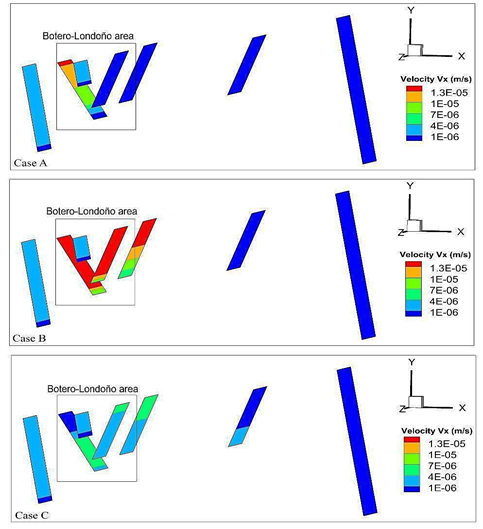
Fig. 7 shows the results for the three scenarios listed in Table 2. The figure focuses on the three faults located in the Botero-Londoño area. The x-component of the velocity vector, which is the most significant considering the main direction of regional-scale groundwater flow in the model, is shown.
Source: The authors.
Figure 7 Comparison of x-component of groundwater velocity for three different scenarios of fault aperture in the Botero-Londoño area (2D regional scale model).
In Case A, where the aperture is 0.1 m, the velocity reaches a maximum of 10-5 m s-1 along the Santa Rosa fault, while velocity for the other faults is on the order of 10-6 m s-1. In the Santa Rosa fault, the highest velocity occurs close to the surface and velocity decreases with depth to a minimum value of 10-6 m s-1. In Case B, with an aperture of 1x10⁻³ m, a velocity of 10-5 m s-1 is simulated along the Santa Rosa, El Billar, and Quebrada Negra faults. Case C, with a fracture aperture of 1x10⁻⁵ m, shows a velocity on the order of 10-6 m s-1 along all faults.
The Santa Rosa fault is selected to compare Cases A and B, since it is the fault with the largest simulated groundwater velocity. The difference between the simulated hydraulic heads at the fault extremities is approximately 0.1 m for Case B, and it is less than 0.001 m for Case A. This difference depends on the head at the lower extremity of the fault, because the head applied at its upper extremity coincides with ground surface, where a first-type flow boundary condition is applied. As expected, the increase in hydraulic conductivity is directly related to fault aperture, but groundwater flow velocity is not necessarily greater with larger aperture, since it depends on the hydraulic gradient along the fault plane, highlighting the influence of the assigned boundary conditions.
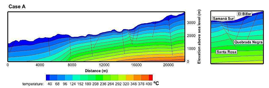
Fault aperture has also an effect on the distribution of simulated temperature since groundwater can flow upward along a fault plane because of hydraulic head gradients (Fig. 8). In Case A, the temperature increases around the Santa Rosa fault while no significant impact is observed along the Quebrada Negra fault. This result is coherent with the work presented by [11], who analyzed the relation between the inclination of the fault and the direction of groundwater flow. Cases B and C, with narrower faults, show a higher temperature at the bottom of the model (438°C for case B and 439°C for case C), which is approximately 50°C greater than Case A.
5.2. 3D Model
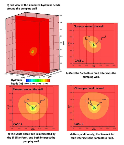
Fig. 9 shows the hydraulic heads simulated in the 3D model. Three different geometric configurations are considered (Case 1, Case 2, and Case 3) varying the mutual intersection between the production well and the three faults, Santa Rosa, El Billar, and Quebrada Negra.
Source: The authors.
Figure 9 Hydraulic heads simulated for three hypothetical scenarios of different fault-well intersections.
Case 1, where only the Santa Rosa fault intersects the well, is characterized by the smallest cone of depression. In Case 2 and Case 3, its extension increases, since the number of intersections between faults and production well increases too, creating a larger network of permeable structures. The three scenarios show that the faults allow withdrawing the fluid from a larger area.
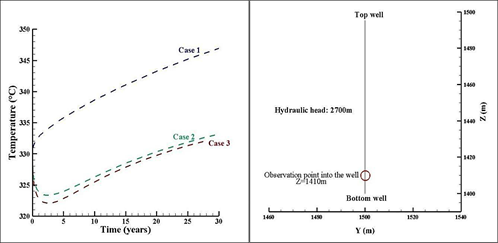
To quantify how the simulated temperature may change depending on the mutual intersection between the faults and the geothermal production well, an observation point is located at a depth of 2590 m, close to the bottom of the well (Fig. 10). The network of permeable structures increases in size from Case 1 to Case 3, because of more intersections between faults and production well (Table 3). Therefore, in Case 2 and 3, the cone of depression is larger (Fig. 9), such that more superficial, and therefore colder, water can migrate to the well. This behavior explains why during the first years of the simulation a small drop in the temperature is observed (Fig. 10), but it is not considered significant to affect the enthalpy of the resource, since it remains in the same temperature range.
Source: The authors.
Figure 10 Location of the observation point at the hypothetical geothermal production well and temperature variation during 30-year geothermal development, for the defined boundary conditions.
Table 3 Description of the 3D simulation scenarios and calculated temperature at geothermal production well.
| Simulated temperature in the well (°C) | Description of the geometry | |
|---|---|---|
| Case 1 | 345 | Santa Rosa fault intersects the well |
| Case 2 | 333 | Santa Rosa and Quebrada Negra faults intersect the well |
| Case 3 | 333 | Santa Rosa and Quebrada Negra faults intersect the well and El Billar Fault intersects Santa Rosa Fault |
Source: The authors.
In Case 1, the average initial temperature around the well is 329°C and increases over time to a maximum value of 345°C, which would increase the geothermal potential. This result depends on the boundary and initial conditions applied. In Case 2 the temperature starts at 329°C, decreases until 323°C in the first 2.7 years, and starts increasing, until it reaches a value of 333°C, which is 16.5°C less than Case 1. In Case 3, the temperature follows the same trend as Case 2, with a small difference of 2°C at the beginning of the simulation, and 7°C at its end.
The analysis of both groundwater flow and heat transfer indicates that Case 2 and 3 scenarios have a similar behavior, which is slightly different from that of Case 1. Scenarios 2 and 3 have a larger cone of depression than Case 1, since the mutual intersections create a larger network of permeable elements (faults and well). This aspect is important to assess the volume of the reservoir that is affected by the extraction of fluids, which is required to identify the proper location of the reinjection well, for example.
The results have shown that the hydraulic and thermal properties, as well as the geometry of the main structures, faults and well, significantly affect the physical processes evaluated. The 2D model shows that the superficial deposits in the zone do not have a representative thickness to affect the assessment of temperature at depth.
The faults in both models are assumed to be open and continuous structures, such that groundwater can flow freely and unrestrictedly by their high hydraulic conductivity. This hypothesis is made because there are no studies about their spatial continuity at depth.
The 3D model was built for the Botero-Londoño zone for two main reasons. First, the faults (Santa Rosa, Samaná Sur, and El Billar) in this zone that are less than 1220 m apart creating a greater fracturing and allowing groundwater to ascend with less restriction, since several hot spring manifestations are observed along Las Nereidas stream. Second, this area is a valley, such that it would be a suitable location for geothermal well drilling, since it would not be necessary to drill across the quaternary eruptive and superficial deposits. It is therefore appropriate to provide new knowledge and insights about subsurface flow and heat transfer mechanisms in this study area, considering that it can also be applied to other regions with analogous geological context.
A limitation of this study is that the variations of water density and viscosity with temperature are neglected, and the fluid is in the liquid phase only. However, the hydrothermal reservoir associated with the NRV is expected to be a liquid dominant reservoir, with a water-steam mixture. Therefore, a more realistic representation should consider two-phase fluid flow (liquid and vapor) and temperature-dependent water properties. However, numerical modeling is generally performed in successive stages, increasing the degree of complexity during time, and this study offers an initial insight into the importance of the intersection between faults and production well. Further modeling tasks can use these results and gradually increase the complexity of the model, to assess the impact of simulating more detailed physical processes. Moreover, considering the numerous available numerical codes, new models may focus on the analysis of different geometrical representations of fractures, using different meshing algorithms. Since a 3D hydrogeological numerical model of this area has not been reported in the literature yet, this study provides useful guidelines to model the available geothermal resources.
6. Conclusions and recommendations
This work presents two numerical hydrogeological models of groundwater flow and heat transfer of the geothermal reservoir of the Nevado del Ruiz Volcano (Colombia). The models focus on the intersection between the faults Samaná Sur, Santa Rosa and El Billar, in the zone called Botero-Londoño.
The results of the 2D model illustrate the impact of fault aperture on the fluid mass balance, as well as on the temperature distribution.
The results of the 3D model show that the spatial distribution of faults has a considerable impact with respect to the cone of depression around a hypothetical production well. Three scenarios with different networks created by the intersection between faults and well, show a relation between the size of this network and the cone of depression associated with withdrawal from the reservoir. The cone of depression explains the temperature observed at the pumping well.
It is recommended to perform geochemical exploration studies coupled to hydrogeological modeling, to define the origin and age of the water and identify the main circulation systems, either deep systems associated with the NRV magmatic chamber or shallow waters. Moreover, geophysical studies can help to improve the understanding of structural geology to better characterize the faults, since their depth, extension, and aperture play an important role for heat transfer and groundwater flow.
With respect to numerical modeling, considering two-phase flow is also recommended for further studies, since it is one of the most important characteristics of a liquid-dominated reservoir, as should be the case in the NRV geothermal system. Two-phase flow modeling would be required once the type of geothermal resources have been confirmed through deep exploratory wells. At that time, it is also recommended to model the geothermal doublet, both production and injection well, to simulate the whole cycle of geothermal resource utilization, to suggest a suitable withdrawal rate to ensure its renewal.
Geothermal energy is a renewable energy if and only if the initial conditions of the hydrothermal system are preserved over time. It should be mentioned that geothermal fluids could present a great diversity of dissolved and precipitated minerals that are neglected in this study, since hydrogeochemical aspects are not simulated. Those minerals are important because, due to changes of temperature and pressure, they can precipitate and cause clogging in wells and pipes of power plants. This phenomenon is another aspect that should be considered and could be analyzed through numerical simulations. Finally, it is recommended to use the 2D models available for this study area to build or update existing 3D conceptual models [17] with the purpose of creating a regional numerical model of the NRV, which can be used to simulate different scenarios of geothermal development.

