Samples

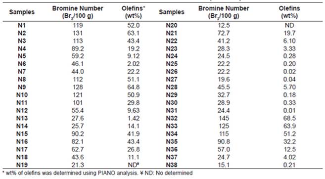
Thirty-eight Colombian naphtha samples were used in this work. Conventional bromine number analysis was determined by electrometric titration (ASTM D1159) ¹⁰. One Mettler Toledo model T90 titrator was used. The temperature for the analysis spanned 0-5ºC, according to the standardized method. Table 1 shows results of bromine number and olefins obtained via the ASTM method.

Acquisition of NIR Spectra

FT-NIR spectra were recorded on a Bruker VERTX 70v spectrometer with a spectral resolution of 8cm^-1 over the range of 4000-13500cm^-1, at 20±0.1⁰C and 32 scans acquisition. Despite the fact that in the majority of works the acquisition of spectra is reported with 4cm^-1, the aim of selecting a resolution of 8 cm^-1 was to reduce the acquisition time to one-half, an important aspect for analyzing a high number of samples. The spectrometer is equipped with a deuterated L-alanine doped triglycine sulfate detector (DLaTGS) and a transmittance sample cell of quartz with 0.5mm optical path. The acquisition time for 32 scans was approximately 30s.

The background spectrum of air was collected for every sample before the analysis in the single beam mode. The spectral files were transformed to ASCII format using the IR Solution software and exported to The Unscrambler software, version X. Five naphtha samples were randomly chosen; ten spectra were recorded for each sample on ten different aliquots. Standard deviation determined was approximately 1x10^-3 (in absorbance units) for any wavenumber.

Principal components analysis

PCA permits to find out samples pattern and which spectral intensities contribute most to this difference. PCA was done through the Unscrambler Software Version X by using Nonlinear Iterative Partial Least Squares algorithm (NIPALS). This algorithm handles missing values and is suitable for computing only the first few factors of a data set. The low information was extracted from the three principal components.

Table 1 Bromine number and w% of olefins in naphtha samples. 

PLS regression

PLS-R was used to establish the relationship between NIR spectral intensities and the bromine number of naphtha samples. PLS-R is a useful procedure to find a common structure between one or more characteristic properties of the samples, called independent variables or simply Y variables, and the spectral intensities, called dependent variables or X variables. In our case, the bromine number in the naphtha samples is the Y variable, while the NIR spectral intensities are X variables. The linear PLS model finds a few variables, which are estimates of the latent variables (LVs) or their rotations. These variables are called X scores, and they are predictors of Y, and also model X; i.e., both Y and X are assumed to be, at least partly, shaped by the same LVs. X scores are estimated as linear combinations of the original matrix of X variables with the weighted coefficients, ^_Wka* (a = 1, 2,..., A). This could be more clearly seen in Equation 1.

Where k denotes the number of X variables or spectral intensities, and i is the number of samples ¹⁹. The regression model can be written according to the Equation 2

meaning that the observed response values are approximated by a linear combination of the values of the predictors. The coefficients of that combination are called regression coefficients or b coefficients. These coefficients are calculated from X scores and Y score. A deeper analysis of the relationship between scores is beyond the scope of this paper, but it is correctly explained by Wold et al. ¹⁹. Regression coefficients summarize the relationship between all predictors and a given response. For PLS, the regression coefficients can be computed for any number of components; i.e., for every latent variable, there are different b coefficients. When X variables have been centered, all predictors are brought back to the same scale; the coefficients show the relative importance of the X variables in the model. Predictors with a the regression model; a positive coefficient shows a definite link with the response, and a negative coefficient indicates a negative relationship. Predictors with a small coefficient are negligible.

Multiple Polynomial Regression (MPR)

MPR is a particular form of linear regression in which the correlation between independent variable X and the dependent variable Y is considered as an nth order polynomial. In a view to performing the regression, principal components (PC) for each sample were used as independent variables and bromine number (BN) values as dependent variables. So, multiple polynomial regression can be represented by the following Equation;

Where air (i,j = 1, 2, 3…) are the coefficients that model the relationship between BN and PC for each sample ²⁰. The goal of MPR is to determine the values of air and minimizing the error, ε.

NIR analysis

Figure 1 shows the NIR spectra of naphtha samples, all showing very similar spectra. In Figure 1, it is though to differentiate between the NIR spectra of heavy and light naphtha samples. However, it is possible to find small differences in the region spanning from 4400-4800cm-1, in particular between the heaviest and light naphtha samples. The bands spanning the region 4400 to 4800cm-1 region correspond to a combination of the fundamental vibrational modes =CH- stretch and C=C stretch. Also, appreciable differences in the region spanning from 5200 to 6500cm-1 can be observed, due to overtones of the vibrational modes corresponding to asymmetric and symmetric stretching of C-H bonds in methyl and methylene group in aliphatic and aromatic compounds. However, even though it is posible to differentiate the naphtha samples through six bands located at 4258, 4335, 4393, 5716, 5866 and 6113cm-1, only after modeling is it possible to know if these differences are associated with the Y variable (bromine number).

Figure 1 NIR spectra of naphtha samples. 

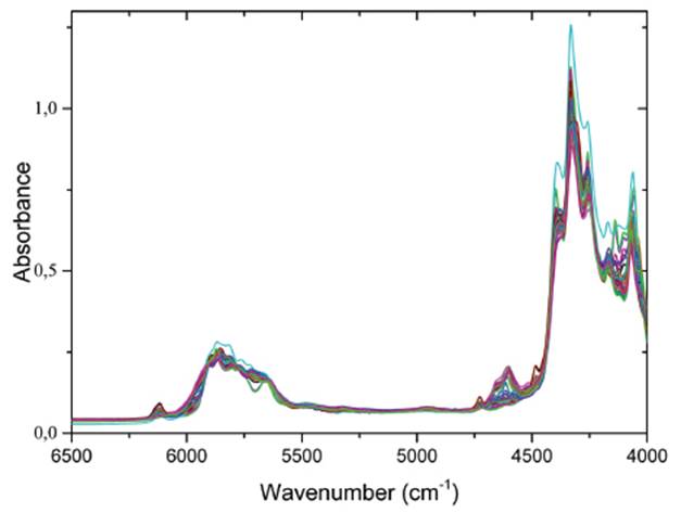
Figure 2a and 2b shows average FT-NIR spectra of heavy and light naphtha samples in the 6500-4000cm-1 range. The overall spectral features were similar to each other. However, slight differences are observed around 4600cm-1, corresponding to aromatic bands. Light naphtha samples show a higher concentration of aromatic compounds. These bands corresponding to olefin compounds, particularly from a combination of =C-H stretching at 3100-3000cm-1 and C=C ring stretching at 1600-1450cm-1.

Figure 2 Average of FT-NIR spectra of (a) heavy and (b) light naphtha samples, respectively. 

Principal component analysis

Principal component analysis was performed using three spectral regions: 4000-4800cm^-1, 5200-6350cm^-1, and 4000-6350cm^-1. In all cases, the first three PCs explained more than 85% of the total variance. These three PCs were used as X-variables in multiple polynomial regression. Figs. 3 show the PCA performed on the three spectral regions.

The plots show two perfectly distinct groups of naphtha samples; twenty-four heavy naphtha samples with a range of bromine number spanning from 12.5 to 72.7 and a group of fourteen light naphtha samples with bromine number between 82.1 and 145. However, N14 y N32 have BN values out of this range. According to Figure 3a, 3b, and 3c, the N32 sample could be considered an outlier, while N14 has a percent of olefin similar to samples in the first range (Table 1). The discrimination between heavy and light naphtha samples occur in PC1; for the region spanning from 4000 to 4800 cm^-1, heavy naphtha samples have negative values and light naphtha samples have positive values of PC1, while for the region spanning from 5200 to 6350cm^-1, heavy naphtha samples have positive values and light naphtha samples negative values of PC1. The behavior of PC2 is entirely contrary.

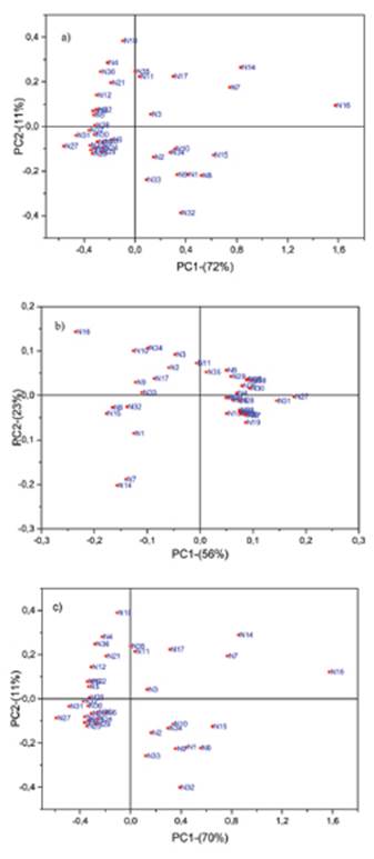
Figure 3 Scores plots of principal components PC1 and PC2 of thirty-eight naphtha samples in the region (a) 4000-4800cm^-1 (b) 5200-6350cm^-1 and (c) 4000-6350cm^-1 

Figures 4a and 4b show loading for PC1 of NIR spectral regions from 4000 to 4800cm-1 and from 5200 to 6350cm-1. As mentioned above, the bands in the spectral region between 4000 and 4800cm-1 mainly correspond to a combination of the fundamental vibrational modes C=C stretch of olefins in naphtha samples. While the spectral region from 5200 to 6350 essentially corresponds to overtones of the vibrational modes of symmetric and asymmetric stretching of C-H and =CH- bond in saturated unsaturated aliphatic compounds. Therefore, the first principal component (PC1) may be attributed to the olefin part in naphtha samples and the second one to aliphatic compounds.

PLS analysis

Intensities from FT-NIR spectra and bromine number for the studied naphtha samples were correlated using PLS regression. After dividing samples into the two groups, i.e., light and heavy naphtha samples according to PCA results, PLS regression was employed to build quantitative calibration models for each group.

Table 2 PLS calibration and validation results for bromine number analysis 

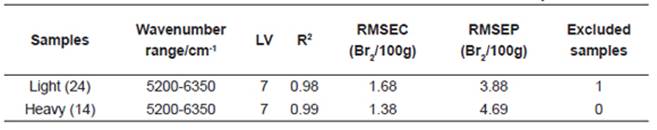
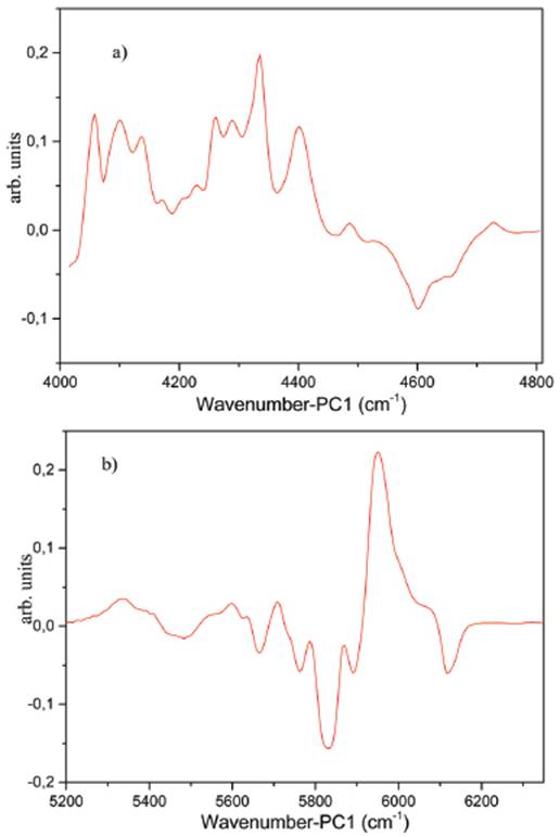
Figure 4 Loadings for PC1 of NIR spectral regions from (a) 4000 to 4800cm^-1 and (b) 5200 to 6350cm^-1. 

The spectral region that best related to BN was between 5200 and 6350cm^-1. The development of predictive models was conducted in two stages; the first one consisted of building calibration models (Fig.4), and the second stage was the validation of the models. The evaluation of the calibration performance was assessed by the root mean squared error of calibration (RMSEC). The standard root mean squared error of prediction (RMSEP) for validation gives an evaluation of the predicted performance of the quantitative model obtained previously. The RMSEC and RMSEP were 1.68 and 3.88 for light naphtha samples, and 1.68 and 4.69 for heavy naphtha samples, respectively. The RMSEC and RMSEP are shown in Table 2 together with the NIR spectral regions, explained variance and factor numbers employed. In all cases, seven factors were used and just one sample (N17), in the model for light naphtha samples was eliminated as an outlier. When the spectral region from 5200 to 6350cm^-1 was selected, the best RMSEP was obtained. If many variables (all wavenumber signals) are used, the model may be unstable; it means that small changes in the spectrum of the order of the spectral noise may produce statistically significant changes in the prediction. These results found in this research indicate that the NIR spectral data can be actually used for the bromine number estimation of naphtha samples.

Figure 5 Number of Principal factor versus RMSE. 

PMR

To compare with PLS-R, multiple polynomial regression calibrations (MPR) was obtained. We used the same wavenumber range selected for PLS-R. Three first principal components (PC), were used as X variables and they explained more than 85% of the data variance. Figure 5 shows the best results when a third order polynomial function and twenty terms (PC1 PC2 PC3 PC1PC2 PC1PC3 PC2PC3 PC1² PC² PC3² PC1PC2PC3 PC1²PC2 PC2²PC3 PC3²PC1 PC1²PC3 PC2²PC1 PC3²PC2 PC1³ PC2³ PC3³ 1) were used. The RMSEC value is 7.44Br₂/100 g.

This value is very high compared to the one obtained via PLS-R. It is possible to use a fourth order polynomial function. However, thirty-five terms will be necessary. When a fourth order polynomial function is used, RMSEC can be decreased to as low as 1.00; however, this result can be due to over-fitting. The preceding results show that the spectral data-bromine number property relationship is linear.

Figure 6 Scatter plots of NIR-PLS prediction values vs reference values for BN both in calibration (blue) and validation (red). (a) Light naphtha samples; (b) Heavy naphtha samples.