


 text in
  English (pdf)
 Article in xml format
 Article references
 Send this article by e-mail
 Cited by SciELO
  Cited by Google
  Similars in
SciELO
Similars in
SciELO  Similars in Google
 Permalink
Introduction
Empirical evidence arises from the accumulation of information that may be obtained through observation of various phenomena or their documentation, even if it is not organized and systematic. It is related to scientific evidence; however, not all empirical evidence meets the strict standards of the scientific method 1.
The scientific method begins with skeptical observation of a known or unknown phenomenon, to analyze it within its real context, uninfluenced by prior beliefs or experiences, after which a research question is posed. Subsequently, it's appropriate conceptual framework is determined and, based on this, a hypothesis is generated that must be tested in an experiment, with results analyzed and conclusions drawn. The reproducibility of the latter allows greater confidence in the result 2.
At this point, it is important to keep three terms in mind which may be used interchangeably but have slightly different meanings: reproducibility, replicability and repeatability. Reproducibility is defined as consistently obtaining the same results using the same data, computational steps, methods, codes and analytical conditions, and is a synonym of computational reproducibility. It also refers to using the same procedure and measurement system, under the same operational conditions at a different site, and therefore is often confused with replicability (different group, different experimental configuration). Replicability refers to consistently obtaining similar results through different studies that analyze the same research question with their own data (different group, same experimental configuration). Repeatability is the least used term and refers to obtaining the same results to determine precision, done by the same research group, under the same conditions (same group, same experimental configuration) 3.
Scientific evidence has developed in the health field due to the systematic observation of the health-disease phenomenon by great masters, who have described it in its various phases. This has led to the development of techniques and methods that can draw us closer to the elusive truth with the lowest possible uncertainty, giving rise to the architecture of scientific research. All of this has resulted in the need to change from the laboratory setting and animal experimentation to the inclusion of human beings as study subjects, in order to make decisions based on etiology, distribution, diagnosis, prognosis and treatment, marking the beginning of clinical epidemiology 4.
Classification of the types of clinical research
The clinician, therefore, needs information to determine the true efficacy of alternative treatments with the lowest possible uncertainty. The taxonomy of scientific literature has established a hierarchy to classify the various types of studies (Figure 1). Describing the type of study is relevant to avoid mistakes in the interpretation and scope of the results 5.
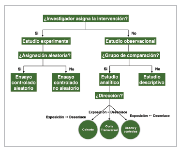
Figure 1 Classification of the types of clinical research (Taken and adapted from: Lancet 2002; 359:57-61).
The study design should be consistent with the type of question defined. Descriptive studies are reserved for new or unknown diseases, which may begin with a simple case report or case series. Cross-sectional studies are aimed at determining prevalence, as they measure the exposure and outcome simultaneously. Case-control studies are important for rare diseases, looking retrospectively from the outcome to the exposure; their main difficulty lies in choosing an appropriate control group. Cohort studies maintain a logical sequence from exposure to outcome; they are important for determining the natural course of the disease, detecting risk factors, establishing the prognosis and studying interventions, to generate hypotheses and show their real-life behavior.
To evaluate the effectiveness of the interventions, observational studies should handle the confounding variables that bias the association by being related to both exposure (in this case, a treatment) and the established outcome. For this, multiple regression, pairing or stratification methods are used; however, these techniques only adjust for observed or known confounding factors. Other techniques have been developed, like the propensity score and instrumental variable analysis. The latter has the benefit of controlling for not only residual confounding but also selection bias, as a study subject may receive a given treatment due to his/ her individual characteristics; for example, the presence of one or more comorbidities, disease severity and prognosis, among others 6. In these cases, correlation is generally shown, not causality, although investigators and clinicians tend to mistakenly interpret it as the latter, when analyzed without the appropriate context 7; the E-value sensitivity analysis could be of help here. It is important to note that we may occasionaly find causality without a clearly observable correlation.
A randomized controlled clinical trial (RCT) is an experiment to evaluate interventions in human beings, understanding "experiment" to be a series of systematic observations, under conditions controlled by the investigator, which are prospective and comparative, since a control group is included which may be active or inactive, such as placebo. In this case, the investigator controls the factors that can affect the variability of the outcome, selection bias, inconsistent application of an intervention and incomplete or biased evaluation of the outcome. In non-experimental studies, the subjects are exposed to interventions for reasons not controlled by the investigator.
Some considerations and criticisms regarding the external validity of traditional clinical trials, especially in the randomization process 8, in line with the availability of enormous databases that show the real-world effect, coupled with the availability of new analytical tools, have led to common sense and clinical observation being proclaimed the preferred methods for supporting clinical decisions. However, more than four decades of experience with well-designed and conducted clinical trials contradict this undesirable practice 9. It is important to note that clinical trials nested in cohorts can be performed when large databases are available.
For these reasons, RCTs (primary studies) are classified as the top of the evidence pyramid, together with clinical trial meta-analyses (secondary studies) (Figure 2) 5.
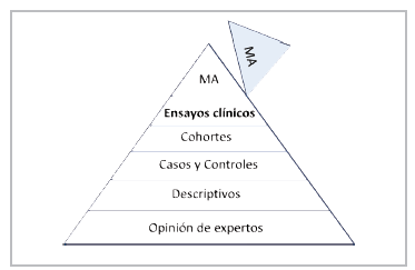
The idea of synthesizing the body of evidence mathematically is very logical and attractive for classifying it at the highest level. However, despite being well developed and conducted, their results depend on the design of each original study, the inherent clinical heterogeneity and methodological aspects 10. The meta-analyses of observational studies are not comparable to those of randomized clinical trials. Therefore, it is important to use systematic reviews and meta-analyses as lenses through which to observe and carefully analyze the body of scientific evidence 11.
They tend to be misused when they are used to "dilute" the negative results of mega-clinical trials designed to answer a clear research question, mixing them with previous studies that did not achieve categorical results, or to highlight effects on specific subgroups, which only serve to generate a new hypothesis. The combination of two or more databases by the same researchers, with no clear structure and design, cannot be considered a true meta-analysis; this falls far short of a meta-analyses performed with data from individual participants (since the former are generally done with grouped data).
Ethical principles
Human subjects research is guided by inviolable ethical principles for their proper participation; these are basically three: respect for people, beneficence and justice. Respect for people refers to their autonomy to participate after discussing the study's conditions and perspectives, and the protection of people with reduced autonomy. Beneficence refers to the obligation to maximize the benefits in light of scientific knowledge and, therefore, minimize harm. Justice is the obligation to treat each person with what is considered to be morally correct and appropriate, as established in the CIOMS guidelines on biomedical research ethics 12.
As Osler stated, medicine is the science of uncertainty and the art of probability. At this point, it is important to introduce the term equipoise, which can be related to the term uncertainty. According to this ethical principle, patients should receive the best available treatment option in terms of effectiveness, according to their clinical condition and individual characteristics. When there are various options, these should be "comparable;" however, clinical trials randomly assign the treatment without considering these variables, based solely on some inclusion and exclusion criteria.
This poses a dilemma between the benefit for the population and advancement of knowledge itself, due to the results obtained, and each patient's individual interest. It is important to establish the biological plausibility of the effect and uncertainty regarding its real efficacy, as it is unethical to conduct studies without a solid experimental backing to predict a successful result with acceptable probability, or if the treatment's benefit is clear ahead of time 13. Another, no less important, aspect in clinical trials is that they should substantiate their scientific and social value.
Clinical research phases
Classically, trials are classified in Phases I to IV, which does not mean that in some cases they are mutually exclusive (Figure 3) 14.
Phase I studies are typically represented by pharmacological evaluation of molecules in healthy people. In general, the following aspects are evaluated: estimated safety and tolerability, pharmacokinetics, pharmacodynamics and the action of the substance or its potential therapeutic benefit.
Phase II studies are usually initial exploratory therapeutic studies. They may have different designs and include control groups or comparisons with the initial status, and they include a homogenous population with very strict monitoring criteria. Their most important objective is to determine the dose and regimen to be administered in Phase III. Some use the Phase IIa subdivision for determining the dose and safety, and IIb for determining efficacy.
Phase III studies are designed to prove or confirm the preliminary evidence obtained in the initial phases, especially Phase II. They include a broader population, may explore dose-response, different disease stages, different scenarios and/or combinations with other drugs. They are considered confirmatory.
Phase IV studies begin when the medication has been approved for marketing, to monitor its effects when applied to an open population that can potentially benefit, and for the indication established in the drug registration.
Common designs of Phase III clinical trials
The design of clinical trials is basically determined by the solidity of the previous evidence of the possible effect. One of the most used designs is that of parallel groups, in which a group of patients is randomly selected to be assigned to one of two or more interventions. This comparison can be made with a placebo control group, when there is no usual therapeutic alternative, or against active treatment if there is a standard therapy. A comparison can also be made between a combination of standard therapy plus placebo against standard therapy plus the experimental intervention, or suspension of the therapy being evaluated against its continuation, in the case of interventions used based on prior evidence with poor methodological quality 15.
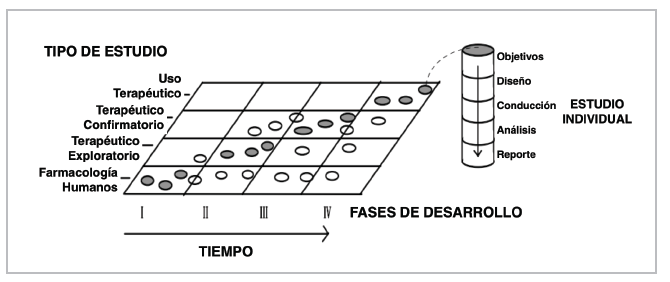
Figure 3 Clinical trial phases (Taken from: International Harmonised Tripartite Guideline: General Considerations for Clinical Trials).
In these protocols, it is not uncommon to use a period in which all patients are exposed to the effect of the intervention prior to being randomly assigned, to evaluate tolerability, also known as a "run-in" period. This increases internal but decreases external validity, as the population included in the trial is selected even more. A similar situation occurs when a significant number of subjects who meet the criteria are excluded for reasons unrelated to the protocol (for example, the attending physician's decision, sometimes due to using the same intervention outside of the RCT). A sham protocol may also be used for invasive interventions, simulating use in all patients to control for the bias induced by the patients themselves, with evaluation separate from the outcome to avoid investigator bias. Likewise, a "double dummy" technique can be used for interventions with different regimens and dosing (every 12 hours vs. every 24 hours or parenteral vs. oral administration), in which the treatment plus placebo is used to replace or simulate the administration of one of the interventions, making them indistinguishable.
Usually, RCTs randomize study subjects to one of two intervention groups; however, they can be designed with multiple arms, in which various elements are combined to answer the research question. These could include comparing various interventions, combining active treatments, different doses of the same intervention, a placebo, a non-active intervention or the usual or standard treatment. There are different analysis options as, for instance, treatment A1 vs. A2 vs. A3 can be compared, if they are different doses of the same intervention, or A vs. B vs. C, if they are different molecules or one of the groups is a placebo. Using several arms increases the possibility of finding efficacy in one of them, improves enrollment and is less expensive.
This type of RCT design includes factorial 2x2 trials, which can compare two different, unrelated (non-interacting) treatments by randomizing the patients twice, once to treatment A and the control and the other to treatment B and the control. Two RCTs for the price of one. Another design used is that of crossed groups, in which the included subjects receive both interventions, but the order in which they receive them differs according to the group to which they are randomly assigned, with a "washout" period before changing the intervention. Less frequently used designs include group or cluster, N of 1, adaptive, and pragmatic designs. The most common are the crossed group (61.3%) and parallel group (24%) designs 16.
According to the purpose of the study, RCTs can classified as: superiority, non-inferiority or equivalence. Traditionally, RCTs have been conducted to prove that a new treatment is better than the standard treatment or the placebo (superiority). In these studies, the null hypothesis (H0) indicates that the new therapy is equal to (generally not better than) the standard treatment/placebo, while the alternative hypothesis (H1), what the study is trying to prove, is that the new treatment is different (is usually better) than the standard treatment/placebo (H0: μ1= μ 0 vs. H1: μ1 # μ0; μ = mean). If the results reach statistical significance, the null hypothesis is rejected, and the alternative is accepted 17.
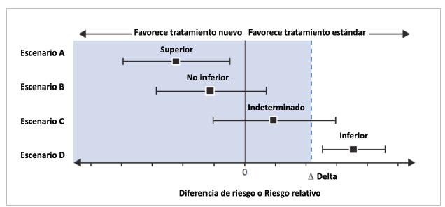
More often, we see RCTs which intend to prove that a new treatment is not inferior to the standard. The new treatment has some advantage over the classic treatment (for example, fewer side effects, greater safety, easier administration or dosing, being less invasive, less expensive, etc.), but maintains a significant percentage of its effect 18. Thus, these studies are not very understandable when the treatment is compared with a placebo, on the grounds of evaluating safety, a strategy used in evaluating some diabetic drugs. The null hypothesis is that the new treatment is inferior to the standard, and the alternative is that it is not inferior (H0: μ1-μ0≤-δ vs. H1: μ1- μ0> -δ; δ: delta, with δ ≥ 0).
An important and crucial point is to determine the known noninferiority margin, or delta, for the primary outcome. This margin represents the smallest difference accepted between the treatments for noninferiority to be declared. The new treatment is expected to maintain at least 50% of the effect demonstrated in previous RCTs of the intervention group versus placebo. The margin determines the possibility of declaring the intervention to be noninferior, and the study sample size (inversely proportional to the square root of the selected delta). Therefore, it should be properly weighted to avoid making mistakes 19-20 (Figure 4). The reevaluation of some of these studies or comparison with subsequent cohorts has shown that many had significant methodological failures, especially in the choice of delta 21,22.
A predetermined sequential strategy can be used in which, if the intervention's noninferiority is confirmed, the study will go on to evaluate superiority. Although the opposite process is possible, its results are unreliable, since the experimental basis on which the intervention's superiority was assumed to be proven has been challenged by the observations, and it communicates a desperate attempt to "save" the trial.
Finally, equivalence studies attempt to prove that the intervention is at least similar to, not exactly the same as, the standard treatment, and therefore also require a prespecified tolerance margin of tolerance. It can be considered an intersection of two non-inferiority trials (H0: μ1-μ0≤-δ and μ0-μ1≤-δ vs. H1: μ1-μ0>-δ and μ0-μ1>-δ) 19.
Characteristics of a clinical trial
A randomized clinical trial is the most rigorous way to establish a cause-effect relationship, with the least possible uncertainty, between the efficacy of one intervention and a defined outcome.
It has important defining characteristics, such as: 1. Random assignment to the intervention; 2. The investigator and study subjects are unaware of which treatment the subjects are receiving, that is, they are blind; 3. The groups are treated the same, except for the experimental intervention; 4. The study subjects are analyzed in the same group to which they were randomly assigned (analysis by intention to treat); and 5. The analysis is focused on estimating the size of the difference in predefined outcomes between the intervention groups 23.
Randomization tends to produce comparable study groups with regard to both known and unknown risk factors, and therefore reduces investigator bias in assigning participating subjects. It also ensures that the statistical tests have a valid false positive rate.
Bias in clinical trials
Bias is defined as the systematic tendency to skew an estimate away from its true value. This skewing can lead to underestimating or overestimating the true effect of an intervention. The various types of bias are selection, performance, detection, attrition, notification and report bias. There are many other types of bias, some of which are directly related to study design and some not, such as accidental bias, in which randomization does not achieve a proper balance in the risk factors and/or prognostic covariables 8.
Selection bias occurs when potentially eligible subjects are excluded, causing a systematic difference between the study groups. All of the study subjects should have a defined probability of being assigned to a specific intervention group. This assignment should not be determined by the investigator, nor should there be a predictable assignment pattern. To avoid this, random sequence generation and blinding of the assignment should be considered 24.
Sequence generation refers to the method used to randomly assign study subjects to each intervention or treatment group, thus balancing the baseline characteristics between groups. Blinding refers to the method used to avoid anyone being able to predict the patient's assignment to a certain treatment group.
There are various random assignment methods, classified as fixed and adaptive. The fixed methods include simple randomization, like tossing a coin, which can produce an imbalance of important factors; block randomized exchange, in which a number of intervention blocks are determined and the order of the interventions in each block is randomly assigned and may vary to avoid being predictable; and stratified randomization, in which a balance of previously determined key factors is ensured, which generally always includes the study center, but may include other variables like diabetes mellitus, age or sex. Overstratification, with the creation of multiple strata, should be avoided 25. Adaptive strategies are less frequently used, with the most well-known being minimization and urn randomization.
Blinding is important for dealing with performance and detection biases. When the participant is blinded, a psychological response to the intervention is less likely, there is a higher probability of following the study regimen, the search for additional or complementary interventions decreases, and withdrawal with no outcome data is less likely. Evaluator blinding reduces bias in the evaluation of the outcome of interest, and investigator blinding reduces the likelihood of investigators transmitting their inclinations or attitudes regarding the intervention to the participants, administering co-interventions differentially, suspending the intervention differentially, adjusting the dose differentially, or encouraging or discouraging participants' continuation in the study 26.
In some cases, blinding is complicated, as in the case of major surgeries; however, even in these cases, false or sham protocols can be developed in which part of the intervention is carried out in both groups (for example, a surgical incision), with the evaluation performed by an investigator who is unaware of who underwent the complete surgery 26,27. The ethical aspects of this strategy have been sufficiently discussed and justified.
Analysis by intention to treat
There are different traditional approaches to evaluating the treatment's effect in RCTs. The recommended strategy is the intention to treat (ITT) analysis, in which each patient is analyzed in the group to which he/she was randomly assigned, regardless of the treatment received, whether that assigned in the study, the control group treatment (crossover) or another available treatment not considered in the evaluation. This strategy allows an unbiased estimate of the effect of the treatment in the entire enrolled population; it is especially unaffected by non-adherence, crossover between groups or potential confounders, as it respects the balance obtained during random assignment 28. However, it can underestimate the actual expected treatment effect in study subjects who were adherent. In other words, if is not used, the effect may be overestimated, even with the named strategies like modified ITT 29.
It is important to note that, in general, non-adherence and intervention crossover are not random phenomena; they have the capacity to affect or not affect the outcome. The ITT analysis is considered conservative in superiority studies but may be more liberal in non-inferiority and equivalence studies, with a tendency to bias the results, making both treatments look similar. Therefore, a per protocol analysis is recommended in these cases 30, especially when the investigators anticipate non-adherence in a significant group of patients (>5%) 31,32.
The alternative is a per protocol (PP) analysis, in which all patients who completed the assigned treatment are included. It excludes patients who violated the protocol, whether because they crossed over to the intervention group or because they never took it. As it does not respect the randomization, it is subject to selection bias by analyzing groups with differences in prognostic variables, similar to a subgroup analysis.
Another option is an as-treated analysis, in which patients are analyzed according to the treatment they received, regardless of which group they were assigned to. This approach skews the effect in any direction, as the effect can be overestimated if the imbalance is due to creating a group with a good treatment prognosis and a better effect or, on the contrary, underestimated if the remaining group has a poor prognosis 29.
Internal versus external validity
The clinical trial is the most appropriate methodological design to answer a research question regarding the efficacy of an intervention. It is important to keep the study's target population in mind to determine with relative accuracy the indication developed from the study analysis, which will be used to establish public health policies for the specific scenario in a broader spectrum (the general population). Defining the target population depends on some established inclusion and exclusion selection criteria, which justify the study question. The stricter these criteria (internal validity), the harder it will be to subsequently extrapolate the results for use in clinical practice (external validity). Internal validity expresses the concordance between the measured effect and the true effect in the population included in the study (sample). This aspect clearly defines the representativity of the selected sample 33.
It is not uncommon to find marked differences between the population included in RCTs and those followed in cohort study registries, in the so-called "real world;" furthermore, there tends to be limited representation of specific groups, such as some ethnic groups, women and/ or elderly patients 34, which limits their external validity (Figure 5).
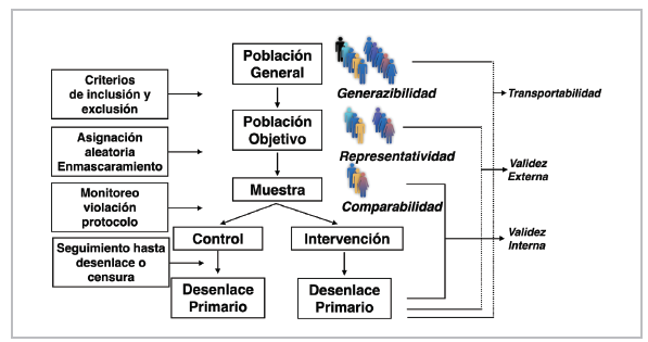
This is not an irrelevant aspect, as some population characteristics can modify the response to certain interventions. Both intrinsic factors like age, sex, weight, ethnic group, genetic burden, biology of the disease itself and comorbidities, as well as extrinsic factors like tobacco and alcohol use and diet, among others, can modify the pharmacodynamics and pharmacokinetics. These factors produce differential and individual responses that must be explored 35.
The purpose of RCTs is to perform causal inference not only on the included sample, but also on a broader population, which will allow clinical application. This allows the results found in the study population to be extended to the target population, as the study population is generally a subgroup of the target population (generalizability). They can also be extended to an external population, with different characteristics (for example, geographic characteristics), allowing their transportability 36,37.
Statistical significance
Statistical significance refers to the simple act of demonstrating that the result obtained within a clinical experiment can be attributed with high probability to a specific cause; in this case, as a result of a medical or surgical intervention. It has mistakenly been interpreted and identified as the result of a statistical test associated with a P value 38.
The P value is an apparently clear and easy target, and therefore widely used, as well as widely abused. We have not finished the argument by mentioning a number of zeros before the 1 (0.0000X1) to highlight the weight of the result of an RCT in academic discussions. There is nothing further from its true interpretation. The cut-off point of P<0.05 is mistakenly interpreted as the 5% probability that a result can be explained by chance or, in other words, that there is a 95% probability of the result being true.
This begs the question: What does the P value mean? The P value is simply the probability that, under a specific statistical model, the summary of the data, like the difference in averages between two compared groups, is equal to or more extreme than the observed data 39. It indicates the incompatibility of the data with the specified statistical model. Under a model constructed with certain assumptions, a small P value indicates the incompatibility of the data obtained with the null hypothesis, which always proposes the lack of effect or lack of relationship between a variable or factor and an outcome (for example, H0: μ1=μ0; μ= mean), whereby it could be rejected, and the alternative hypothesis accepted (H1: μ1≠μ0)..
Determining statistical significance should begin with the proposed experimental design and whether it is appropriate for answering the research question, the scientific basis for the hypothesis to be tested, how adequately the study was conducted, data collection, data monitoring, and exploratory analyses performed under the established statistical model, finally arriving at the P value (the tip of the iceberg). It is common to find the well-known phenomenon of data dredging, selective inference or hacking, which expresses the investigators' attitude of finding associations without the due scientific evidence to support the hypothesis, as it was not previously proposed in the design.
Another phenomenon that impresses the unwary is purchasing the P value. Any effect or association, no matter how weak, can produce very small P values simply due to large sample sizes or using a high precision measurement. The opposite can also be true: significant effects can produce unimpressive P values due to small sample sizes or the use of imprecise measurements. A small P value tells us that the data obtained are unusual under the assumptions of the tested model, but this may simply be due to a false hypothesis or study protocol violations 40.
We must always keep in mind that statistical significance does not represent scientific or clinical significance. For example, a 1% reduction in the level of any variable (blood sugar, total cholesterol, blood pressure) can yield statistical significance with P<0.05; however, the clinician is responsible for interpreting this in light of the knowledge available to decide if the actual effect is relevant on a surrogate outcome or an important outcome. Therefore, the P value does not measure the importance of the outcome nor the effect size 40.
The level of statistical significance also represents the probability of the well-known type I error, denoted by . This error occurs when H0 is rejected but is true. Statistical power is related to the well-known type II error, as the complement of 1-; thus, the statistical power of a hypothesis represents the ability to detect a specified effect size for a given level of significance, in other words, to reject H0 when HA is true (Table 1). Ideally, an RCT should have sufficient power to correctly accept the HA when it is true. Most RCTs choose 80% power.
Analysis and interpretation of the results
The final, no less important, phase is interpreting, analyzing and reporting the results. The presentation should be as clear and concise as possible to achieve an assertive communication that allows the reader to properly interpret the data, weigh the results and reach valid conclusions, in line with what has been shown and published. The investigators are responsible for critically analyzing the results, without giving in to the temptation of drafting the paper in a way that minimizes the risks found and appears more robust than it really is.
The investigators should avoid the not infrequent practice of "spinning" the results to make them benevolent if they were negative or making the study positive by highlighting secondary outcomes, subgroups or post hoc analyses, without due explanation of the fact that they are exploratory analyses that generate a new hypothesis 41.
Neither having been published in a high-impact journal nor having been performed by well-known scientific researchers is an argument to support the given results and interpretation. Scientific journals have a great responsibility in publishing articles; however, millions of articles are submitted for publication every year, in thousands of journals, which makes it especially difficult to choose the best. In addition, peer review is not free from problems like poorly prepared reviewers (many of whom receive no remuneration from the publishing houses), conflicts of interest, and even fraud, not to mention the bias toward publishing positive studies, especially industry-sponsored studies 42.
Sophistication in the development and performance of RCTs has allowed the interpretation of results to be manipulated to impress unsuspecting readers, especially with the use of more complex statistical analysis techniques. Not even the requirement of previously publishing the protocol in different registries or databases has achieved transparency in this aspect, as there are flaws and clear discrepancies between what is registered as the protocol and what is published, which, unfortunately, at times includes changing the primary outcome evaluated 43,44,45.
Although the guidelines are clear, RCT reports in scientific journals tend to be biased toward exaggerating the difference of the interventions in the results. The most common statistical problems include the use of multiple primary outcomes, the use of unrelated primary outcomes, the analysis of numerous or non-prespecified subgroups, the use of repeated measures over time without a predetermined strategy, the use of more than two treatments without an established analysis, the use of numerous statistical significance tests, not calculating the sample size or modifying it with no clear justification, the lack of clear rules for stopping the study (stopping early overestimates the effect), differential cut-off points in the statistical tests, and a biased selection of results in the abstract, including privileging secondary outcomes, even with a negative primary outcome 46,47.
One crucial aspect of RCTs is choosing the appropriate outcome, one with the ability to capture the efficacy of the treatment, whether as a clinically relevant or surrogate outcome. Occasionally, RCTs fail in "betting" on the wrong outcome, for example, a combined outcome or mortality instead of readmission. A surrogate outcome is one chosen for measurement in place of another variable, especially because it can reduce the sample size or length of the study, by replacing an outcome that rarely occurs or that takes longer to occur with one that is more frequent or occurs more rapidly 48,49.
After obtaining a positive result with statistical significance, it is important to determine other aspects that show the robustness of the result. Unfortunately, we often stop at the binary result of whether or not it is statistically significant (P<0.05), without gathering information on other extremely important aspects.
Therefore, we suggest asking some questions:
• What is the effect size?
The difference found between the interventions should be clinically relevant, large enough to be considered significant. It is important to review the estimate used, relative risk or instantaneous risk (hazard ratio), and its confidence interval (95% CI). It is also relevant to determine the difference in the rate of events on follow-up and the number needed to treat (NNT= the reciprocal of the absolute risk difference) 50.
• Is the primary outcome clinically important?
In general, Phase III RCTs use clinical outcomes like mortality, although they may use some surrogate outcomes, which cause controversy. The other important point is the use of combined outcomes, which should be related in some way, pathophysiologically or otherwise, occur with a similar frequency and have a similar impact as the intervention; however, very often the result shows a greater effect on one of them, individually, which makes them hard to interpret. They have the advantage of reducing the required sample size, follow-up time and costs, and may include the net clinical benefit by incorporating adverse events 51,52. Co-primary outcomes, not necessarily combined outcomes, may be used, and a hierarchical analysis can be established to sequentially analyze the defined outcomes using a predetermined hierarchy until statistical significance is lost, at which point the following ones are considered exploratory.
• Are the results consistent?
When using combined outcomes, it is important for the impact of each to be similar and in the same direction. Also, the effect on secondary outcomes should be analyzed, which gives greater weight to the results 50. In the subgroup analysis, it is important to keep certain aspects in mind to avoid a wrong interpretation, giving it a weight it does not actually have. The figure showing the results by subgroups, which is usually at the end of the study report, should be looked at first; in this figure, the estimates should be located on the same side as the one obtained in the total sample (all on the right or all on the left); even if the 95% CI is greater than one, it may be accompanied by an additive or multiplicative interaction P (Figure 6) 53.
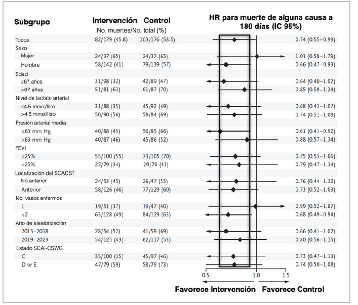
Figure 6 Results by subgroups in RCTs. (LVEF: left ventricular ejection fraction; STEACS: ST elevation acute coronary syndrome; SCAI-CSWG: Society for Cardiovascular Angiography and Intervention- Cardiogenic Shock Working Group). Source: example taken from an RCT published in the New England Journal of Medicine.
Then we must determine if the size of the difference was clinically important, if it reached statistical significance, if the hypothesis precedes the analysis, given the theoretical support for exploring this specific subgroup, if the difference was suggested by the evidence in other studies and was consistent among them, and if the number of subgroups chosen was one of a small group of hypotheses to be tested in the study 54. Generally, they should be considered hypothesis generators 55. Other equally important aspects to evaluate are whether the sample size is large enough to be convincing, as small RCTs with overwhelming results should be taken cautiously, as well as surprisingly low estimates (too good to be true; even if the sample is large), especially if they are not consistent with the results of other studies. Also, whether the study was stopped early (due to efficacy, futility, adverse events or logistical problems), whether there is an appropriate balance between efficacy and safety and, lastly, any evidence of inappropriate running of the RCT, recalculation of the sample size or estimated enrollment period with no justification, the quality of the data, an elevated percentage of losses or missing data that cannot be overcome with multiple imputation, and lack of adherence, among others.
Some interventions have been gaining ground due to their innovative profile or attractive mechanism, but have not been adequately tested in RCTs, and in spite of this, have become part of standard treatment. When an RCT is performed to evaluate these interventions, we are surprised if the results are negative and are particularly reticent to accept them and incorporate them into daily clinical practice. Unlearning is a difficult and complex process.
• What to do when an RCT is negative?
Several critical aspects should be explored, such as whether there is at least a glimpse of a potential benefit. It is essential to evaluate if the RCT had low power; if the proper outcome, population and treatment regimen were chosen; and if there were deficiencies in running the study. It is also necessary to know if a non-inferiority analysis was proposed, if there was some positive sign in subgroups or secondary outcomes that could generate hypotheses; or if alternative analyses could be explored (adjustment for covariates, per-protocol or as-treated analyses, or a competing risks or recurrent events analysis) 56,57.
Estimating the effect of the interventions (part II)
The objective of the statistical analysis of an RCT is to estimate the size of the difference of the interventions on the outcomes; for example, the difference in means between two groups in the selected outcomes. First, a point estimate is determined, which corresponds to the observed difference, and then the degree of uncertainty of the data should be determined, usually using 95% confidence intervals (95% CI) 58.
The type of estimate used depends on the nature of the outcome of interest. There are basically three: 1. Binary (yes or no, living or dead); 2. Time-to-event (survival); and 3. Quantitative outcome (e.g., blood pressure readings) 58.
In acute illnesses with generally short follow-up times, a comparison between two interventions is set up in binary terms as the "absence" or "presence" of a relevant clinical event. The characteristic of the clinical event depends on the setting and disease studied, and can range from mortality (living or dead) to major and minor complications. Thus, the comparison of the groups at the end of the defined follow-up period gains relevance, and the way in which the given event developed throughout the observation period becomes less interesting 58. In these cases, the effect can be quantified through measures like absolute risk reduction, relative risk reduction or the NNT 59.
Risk refers to the probability of an event or outcome occurring; in statistical terms, it is the probability of the outcome of interest over all possible outcomes. Odds refers to the probability of an event occurring over the probability of it not occurring. Although it is a harder term to understand and is often used in the betting world, it is useful when logistic regression models are used to adjust for variables, due to its greater mathematical versatility and conversion to log odds. Odds and risk are commonly confused and used interchangeably; however, they are different concepts, although very similar when the rate of events is <10% (Table 2) 60.
Once the probability of an event is known, the odds can be cleared up. For example, if the probability is 0.2 (the second scenario in Table 2), the odds of the event occurring would be 0.2/0.8=0.25, or the probability divided by 1 minus the probability, 0.2/1-0.2=0.25 (Equation 1). From this, we can deduce that when the probability is small, the odds are almost identical to this probability (for example, a probability of 0.05). The log odds of the event occurring would be: Ln [0.2/0-8]=-1.38 (the logarithm of a ratio is equal to the logarithm of the numerator minus the logarithm of the denominator), or Ln (0.25) =-1.38. The probability can be calculated as odds /1 +odds (Equation 2), that is, 0.25/1.25=0.2 or exp [Ln (odds)]/1 + exp [Ln (odds)]= exp (-1.38) /1 + exp (-1.38) =0.25/1.25. Easy! 61.
Relative risk (RR) refers to the ratio between the rate of events in the intervention group and the rate of events in the control group (exposed/not exposed). The odds ratio (OR) is the ratio of the odds in the intervention group to the odds in the control group. Taking the data from Table 2 as an example, the first scenario would be the control group, and the second would be the intervention group; the relative risk would be 0.2/0.3= 0.66 and the odds ratio would be 0.25/0.43=0.58. The 95% confidence intervals can be mathematically calculated 62. The RR can be calculated from the OR using the formula RR= OR/ [1-P0 + (P0 x OR)], where P0 is the baseline risk of the study population (in the example, it would be P0=0.25) 63.
Table 2 Odds and hazard with different rates of events.
| Intervention | Outcome | ||||
|---|---|---|---|---|---|
| Death (a) | Survival (b) | Total (a+b) | Hazard [a/(a+b)] | Odds (a/b) | |
| First | 30 | 70 | 100 | 30/100=0.3 | 30/70=0.43 |
| Second | 20 | 80 | 100 | 20/100=0.2 | 20/80=0.25 |
| Third | 10 | 90 | 100 | 10/100=0.1 | 10/90=0.1 |
| Fourth | 1 | 99 | 100 | 1/100=0.01 | 1/99=0.01 |
Nota: four scenarios are proposed with different rates of events; N=100 is used to facilitate the calculation.
The difference in outcomes between the groups can be described in absolute or relative terms. In these cases, the terms "absolute risk reduction" (which is simply the difference between the rate of events in the two groups), or "relative risk reduction" (which is the difference between the rate of events in the two groups expressed as a proportion of the rate of events in the control or untreated group, and generally constant across different baseline risks) can be used (Table 3).
Table 3 Relationship between absolute and relative risk reduction according to the baseline risk.
| Risk of the outcome Mortality | ARR | RRR | NNT | |
|---|---|---|---|---|
| Intervention | Control | |||
| 10% | 5% | 5% | 5/10 = 50% | 20 |
| 80% | 40% | 40% | 40/80 = 50% | 2.5 |
| 2% | 1% | 1% | 1/2 = 50% | 100 |
Absolute risk reduction should be interpreted in light of baseline risk and is smaller with lower rates of events, while relative risk reduction remains relatively constant. The lower the rate of events in the control group, the greater the difference between the relative and absolute risk reduction. Both measures should be reported, and the clinician must determine the relevance of the result.
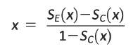
The number needed to treat (NNT) or harm (NNH) expresses the number of patients who must receive the intervention to avoid an outcome; it is calculated as the reciprocal of absolute risk reduction x 100 64. In the first example described in Table 3, 20 patients would need to be treated with the evaluated intervention to avoid one death. We should keep in mind that for binary outcomes, NNT depends on the length of follow-up. This means that there is no single NNT value, but rather several that can be calculated at a specific point after beginning treatment 65.
In an RCT, if the hazard ratio (HR) is available, the NNT could be calculated at a specific point knowing the probability of survival of the control group, using the formula: NNT = 1/ {[Sc(t)]HR - Sc(t)} (Equation 3); where Sc(t) is the probability of survival of the control group at the given time, and therefore the probability of survival of the active group would be [Sc(t)]HR. For example, if the probability of two-year survival is 0.33 and the reported HR is 0.72 (95% CI 0.55-0.92), then the two-year NNT would be = 1/0.33072 - 0.33 = 8.32 (example taken from reference 65).
Time-to-event (survival)
In chronic diseases like cancer or cardiovascular diseases, the time elapsed between exposure (in this case the intervention) and the defined event of interest (usually mortality), becomes important. Mortality and survival are not interchangeable terms, since the first is dichotomous, used to compare two groups within a specific amount of time (30 days, one year, five years), regardless of the interval elapsed, while the second gives importance to the timing of the event, as an essential variable. Ultimately, all will have the outcome; to put it crudely, all study subjects will die, it just depends on the time established for measuring it. Therefore, the time-to-event becomes relevant. Although it was proposed as a survival analysis, the outcome is not only mortality; it may include other outcomes of interest like relapses, readmissions, and progression, among many others.
Despite the mistaken belief that all patients in RCTs are treated simultaneously, study subjects are enrolled over the recruitment period, which may even be longer than the follow-up period. Therefore, it is not unusual for some patients to leave the study before others enter or reach the end of the study without having developed the event of interest 8.
In a survival analysis, the time variable is referred to as the "survival time," and the onset of the event as "failure," precisely because of its negative connotation, although some events could be positive. Survival time is a positive variable with a skew to the right, and therefore a normal distribution cannot be used as a model. Ideally, all the subjects in a study would be followed until the event to establish comparisons. However, the study may end due to the required number of outcomes being reached (we are speaking of sample size, but what is calculated is the number of events needed to obtain the established power), without the subject experiencing the event, and therefore we really do not know his/her complete survival time 66.
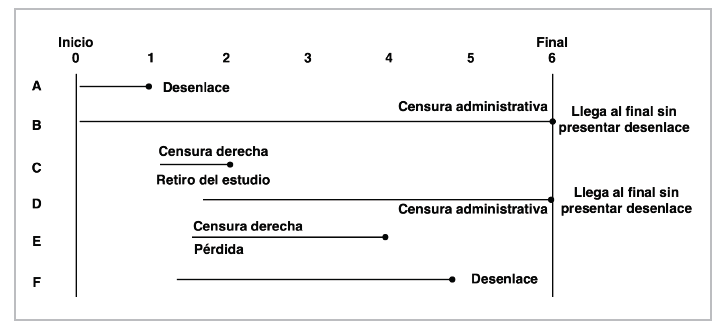
This phenomenon is known as censoring (administrative censoring). There are other reasons for censoring, like losses to follow-up or withdrawing from the study for some reason or having an event other than the event of interest, which is known as competing risks; this type of censoring is known as right-censoring. Left-censoring is rare in trials and is caused by the failure having occurred before study enrollment 67 (Figure 7).
Survival distribution
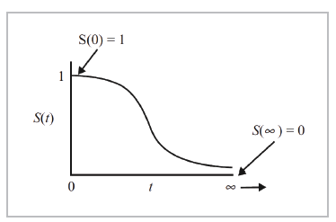
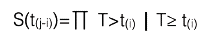
Survival distribution is generally described in terms of two functions: the survival function and hazard function. The survival function, S(t), represents the probability of a person exceeding a specific time "t"; in other words, the S(t) function gives the probability that the random variable T will exceed the specified time t. It is represented by the following equation:
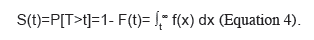
It is a monotonic and decreasing function. Theoretically, since the range of time t is from 0 to infinity, it could be graphed as a curve with a gentle slope (Figure 8).
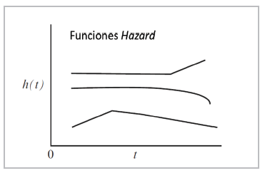
The hazard function, h(t), represents the instantaneous potential (instantaneous risk) by unit of time for the event to occur, given that the subject has survived until time t. This is represented by Equation 5:
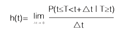
In mathematical terms, the hazard function is a conditional probability, similar to the classical statement of the probability of A, given B [P (AB )]. The probability that a study subject will exceed time T, which will be found in the interval between time t and t, since the survival time T is greater than or equal to t (the numerator in Equation 5) is not so easy. However, the denominator introduces the concept of time, in this case t, which makes it a rate, and therefore its range is not from 0 to 1, like a probability, but rather from 0 to , defined in units of time like years or months 66.
The hazard function can be graphed in a similar way to the survival function, but unlike the latter, it does not begin at 1 and tend toward 0, it begins anywhere (h(t) >0) and increases in any direction, up or down, over time (it has no upper limit). Of the two functions, S(t) and h(t), the survival function is most used. The h(t) function is important because it measures the instantaneous potential, while the S(t) function is a cumulative measurement over time. In addition, the first one identifies a specific model (exponential, Weibull or lognormal) and is the mathematical way to model the survival curve 66,67,68 (Figure 9).
The Kaplan-Meier estimator
In oncology, estimated patient survival is accepted as the main criterion for evaluating treatment effectiveness. It is reported as 1-, 3-, 5- or 10 or more-years' survival. To achieve this, each patient must be followed individually for the established time, using the known survival tables, although it is not uncommon for the course of some patients in a cohort to be unknown because they are followed for a shorter amount of time or are lost to follow-up, which leads to observations with incomplete data. In 1958, Kaplan and Meier published their classic article on estimating survival rates with incomplete or censored data, which became the standard analysis 69. Each research subject contributes a follow-up time to the analysis (until he/she develops the outcome, is lost to follow-up or presents an event other than the event of interest.
We return to the concept of censoring to define random censoring as that in which the study subjects that are censored at time t must be representative of all the subjects that remain at risk at the same time with regard to their survival. Independent censoring expresses the same concept, but within any subgroup of interest. Non-informative censoring determines that the censoring mechanism cannot be related to the time-to-event distribution; for example, it is considered informative censoring when the subject withdraws from the study for a study-related reason, i.e., an adverse event, violating the assumptions on which the survival analysis is based 66,70.
With these concepts clarified, we will now compare two groups of study subjects. First, we tabulate each of their experiences (outcome or censoring), which gives us an idea of their survival at a specific point. Each subject is characterized by three variables: 1. His/her time series (t); 2. His/her status at the end of the time series (censoring [cj] or outcome [oj]); and 3. The study group to which he/ she belongs (Table 4). Calculate the probability of survival for each time (t) (Equation 6) 71.
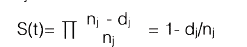
Thus, Kaplan-Meier calculates the probability of survival for each specific time (tj) as a product (Equation 7) that expresses the probability of exceeding the previous time at which a failure (outcome) occurred, multiplied by the conditional probability of surviving past the time (t), since the subject reached at least this time (tj). Not very simple, but it will be with an example!
Survival is calculated for each time tj; the time elapsed between each outcome is determined by an interval Ij, that runs from time t(j-1) to the time of the event t. For each event time, we determine nj, which is the number of subjects who reach this point alive (or without the outcome, if it is not mortality), as well as dj, which is the number of subjects who have the outcome during this interval or cj, if they were censored (Table 5) 67.
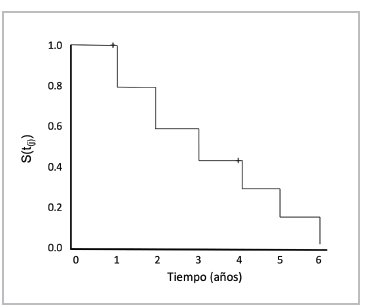
Finally, we can graph the survival curve with this data at times t1, t2, t3...t6, marking the censored observations with a + sign (Figure 10) 72.
Log rank test
We can also graph survival curves for both the intervention as well as the control groups, to give us an idea of their behavior over time, find differences between the two, and even compare the survival proportions at a specific time. However, the full comparison of the survival experience between the two groups throughout the follow-up time is lost. To be able to fully capture this, the log rank test 73 is used, testing the null hypothesis that there is no difference between the populations (intervention and control) in the probability of death at any point. The number of observed deaths and those that would be expected if there really were no difference between them [(O-E)2/E] is calculated for each interval, and the statistical significance is determined in the Chi2 distribution table. The median survival can also be calculated (which is the time at which half of the patients are alive and half are dead), along with the average survival, according to the area under the curves.
Table 4 Construction of a table for a Kaplan-Meier analysis.
| Subject | Time (years) | Status at the end of the period | Group |
|---|---|---|---|
| 1 | 0 | O | I |
| 2 | 1 | C | C |
| 3 | 2 | C | I |
| 4 | 3 | O | C |
| 5 | 4 | O | C |
| X | 5 | C | I |
O: outcome; C: censoring; Intervention; Control
Table 5 Example of the Kaplan-Meier estimator in an RCT intervention group.
| Intervention group | ||||
|---|---|---|---|---|
| tj (years) | nj | dj | cj | S(t(j)) |
| 0 | 18 | 0 | 0 | 1 |
| 1 | 18+ | 3 | 1 | 1 x (1-3/18) =0.834 |
| 2 | 14 | 3 | 0 | 1 x (1-3/18) x (1-3/14) = 0.834 x 0.7857=0.655 |
| 3 | 11 | 3 | 0 | 0.655 x (1-3/11) = 0.655 x 0.727 = 0.476 |
| 4 | 8+ | 2 | 1 | 0.476 x (1-2/8) =0.476 x 0.75 = 0.357 |
| 5 | 5 | 3 | 0 | 0.357 x (1-3/5) = 0.357 x 0.4= 0.142 |
| 6 | 2 | 1 | 0 | 0.142 x (1-1/2) = 0.142 x 0.5 = 0.071 |
Time in years to facilitate the example, but it is determined by the time at which the event occurs; t: time of the event; n: number of subjects who reach the time alive; d: number of subjects with the outcome; c: number of censored subjects; S(t ): cumulative probability of survival.
The log rank test was proposed to give equal weight to all the failure times during follow-up, and therefore assumes a proportional hazard ratio between the groups throughout the follow-up period. However, it is not uncommon for the hazard ratio to vary, in which case one of these other tests should be used, like Gehan-Wilcoxin, Tarone-Ware, Peto-Peto or Fleming-Harrington, among others 74.
Cox regression model
The technique most used for evaluating the relationship between explanatory variables and survival time was described by Cox in 1972, known as the proportional hazards regression model 75. The model describes the relationship between the hazard function (risk of an outcome) and a group of covariables or factors. The equation (Equation 8) is written as follows:
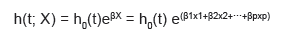
Where h(t; X) is the hazard function for individual i with X values = (xrx2,.. .xp) in the explanatory variables at time t; therefore, it is the variable to model and represents the risk of dying at time t of the study subjects who have a given pattern X of the explanatory covariables; eßX is the exponential function of the p xi explanatory variables with their respective regression coefficient; and h0(t) is the baseline hazard function when all covariables have a value of 0 76.
The baseline hazard function is not specified in the model, and therefore it is not assumed to follow a particular distribution pattern; the effect of the treatment and the co variables is multiplicative; the hazard of the event of interest in a group is a constant multiple of the hazard of the other; the hazard ratio is constant over time (Figure 11); and the survival times are independent among subjects, who have the same risk until the outcome or censoring 76.
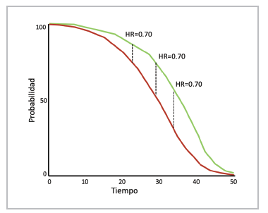
Figure 11 Proportional risk. Two RCT groups: intervention (red) and control (green). The hazards may change, but the hazard ratio is constant.
The semiparametric estimate in the Cox regression is done using the partial likelihood method, although considerable computation times may be required when there are ties (more than one individual with the same failure time), and therefore approximations are used like those proposed by Breslow, Efron and Cox. The proportional hazard assumption must be tested; initially, assessment of the Kaplan Meier curves gives an idea of whether it has been violated, if the curves cross or one of them slopes down while the other ends in a plateau. Then, the so-called Schoenfeld residuals are analyzed, or the log-log plot method, among other tests, is used for confirmation. The effect of a covariable may also change over time, for which a different analysis should be proposed 77,78.
The HR is calculated by the hazard rate, the instantaneous risk rate, in each group included in the trial. The hazard rate is defined as the rate of conditional instantaneous events calculated as a function of time. For example, if a group of 100 patients undergo a treatment and two die after one month, the hazard rate is 2/100; if one patient dies in month two, the hazard rate will be 1/98, and so forth. In this case, the hazard rate is the number of patients who die divided by the number of patients who are alive at the beginning of the time interval. Consequently, HR is the ratio of hazard rates at which the patients in both groups experience the outcome 79.
A common mistake in practice is to interpret HR as the reduction in the risk of the event, as a percentage equal to 100(1-HR); the HR reduction means that the time to the event, for example, death, is extended, not exactly that the event is avoided. An HR of two means that at any given time proportionally twice as many patients in the intervention group have an event when compared with the control group, and an HR of 0.5 indicates the opposite: proportionally half of the patients in the intervention group have an event during any time interval compared with the control group. An HR=0.6 looks very impressive but does not represent a 40% reduction in the risk of events at any time during follow-up. To calculate the risk of the event (x), the survival distribution must be known in both the intervention or experimental group [Se(x)] as well as the control group [S (x)] (Equation 9) 80."
Nonproportional hazards
The proportional hazards model assumes a constant HR (Figure 9). However, given the heterogeneity of the population included in an RCT, it is possible that when both high and low risk patients are combined, a proper balance of covariables will not be achieved, making interpretation difficult despite proving the assumption. This may be caused by the presence of unmeasured (or unknown) covariables, which can affect the outcome 81.
It is assumed that these unmeasured factors are multiplicative on the hazard scale, which is how the Cox regression is parameterized, and therefore the included bias (selection bias) increases with the magnitude of the causal effect, heterogeneity of the baseline hazard and follow-up time. We may find ourselves in a scenario in which the curves diverge early but tend to converge during follow-up. Although this is difficult to explain, it may be due to a gradual reduction in treatment efficacy or survival bias. The other possible scenario is when the curves diverge gradually, which could possibly indicate that the efficacy of the treatment increases over time 81. There are other possible scenarios in which the assumption of proportionality is not met, and therefore alternative strategies must be used for evaluation.
Restricted mean survival time (RMST)
The log rank test and Cox regression model, which allows adjustments for covariables, are robust in the presence of nonproportional hazards, in the sense that they maintain some of the power to differentiate between two treatments whose hazard functions are not proportional. However, in extreme cases, such as the classic example of when the survival curves cross, this power is reduced. Therefore, Royston P. and Parmar M. proposed the restricted mean survival time analysis 82.
In theory, the average survival time can be calculated as the area under the curve of the survival function to infinity (Figure 8), as long as there are no censored observations. Therefore, the median survival time is used more often, which is defined as the time in which half of the patients develop the outcome of interest and requires a significant number of events and follow-up time to estimate. The RMST is similar to the average survival time but, as its name indicates, is restricted to a specific time 83.
The RMST can be defined as the area under the curve of survival of T up to time t, that is, from time 0 up to the time determined by the investigator. Likewise, restricted mean time lost (RMTL) can be estimated, as its complement. The effect of the intervention is determined by comparing the RMST between the groups (intervention and control). For example, with t=40 months, if the area under the curve is 35.4, this means that, on average, future patients exposed to the intervention would be alive (if the outcome is death) for 35.4 of the 40 months of follow-up; the RMTL would be 4.6 months. If, when comparing the two groups, the RMTL is 4.6 months in the intervention group and 6.7 months in the control group, this is interpreted to mean that a patient in the control group would live an average of 2.1 months less (for more clarity, see the example in reference 84).
This analysis allows a simpler, more intuitive interpretation, considers the entire distribution of survival up to the given time, does not require the proportional hazards assumption to be met, and can be used as a complementary analysis in the event that it is met. However, the disadvantages may be that the conclusion of the RMST may vary depending on the time specified for analysis in the case of nonproportional hazards. Therefore, the time interval should be clinically motivated and prespecified in the clinical trial protocol. Also, the RMST delta (difference between groups) may appear to be a relatively small effect as far as the months (or days) of life gained per years of therapy, possibly influenced by relatively short follow-up times 85,86.
Accelerated failure time (AFT)
The literature is evasive in describing this model and its usefulness; it was described in 1966 by Pike MC (87) in the phenomenon of carcinogenesis. It is termed "accelerated failure time" because, similar to other models, the term "failure" represents the onset of the event or outcome, and it is "accelerated" because it is assumed that the effect of a covariable is to accelerate or decelerate the course in a constant manner. The model explains the relationship between the survival probabilities and some covariables, estimating a relative relationship. It provides an estimate of the time-to-event medians, which can translate into a reduction in the duration of the disease 88.
Instead of estimating the hazard ratio, the model estimates the time ratio (TR); the TR estimates the delay until the occurrence of an event, with treatment compared to the control group. For example, a TR of 2 means that the time until an event occurs is twice as long in the intervention group as in the control group. If the HR is 0.71 and the TR is 1.51, the first expresses a 29% reduction in the hazard, the instantaneous risk, of events in the intervention group versus the control (notice, a hazard reduction), while the other expresses that the time to event is delayed by 51% in the intervention group compared to the control. The opposite of TR is known as the acceleration factor (AF); this represents the same effect direction, that is a TR=2 is the same as an AF=0.5, and indicates that the time-to-event is twice as long as the control, as mentioned. It can be expressed in the logarithmic scale (similar to a linear regression) as
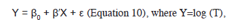
ε is a random error term that is assumed to have a parametric distribution and ß0 is the intercept; there are various types of AFT models, such as exponential, Weibull, log-normal, gamma, and log-logistic, with the latter not restricted to the proportional hazards assumption 89. Since different probability distributions can be adjusted, the one best suited to the data can be selected, using the Akaike information criterion (AIC).
Survival analysis restricted to a specific time (Milestone analysis [MA])
Milestone analysis is defined as the probability of survival defined by Kaplan-Meier in a specific time, ideally established a priori (probability from 0 to 1 or a proportion from 0 to 100%). The method is similar to using logistic regression or calculating the OR. It is recommended that the analysis be done when at least the last cohort subject has reached the time established for analysis. It is used for interim analyses or to evaluate the "tail" in long-term survival 90,91,92. It must be distinguished from the landmark analysis described by Anderson et al., to evaluate bias in the survival analysis when a covariable of interest is, in fact, a study measure like response status (responders vs. nonresponders); in the latter, only subjects who are alive at the time of interest are analyzed 93.
Win ratio (WR)
Compound outcomes are often used in RCTs because they reduce the required sample size, follow-up time and costs. They are generally evaluated with the KM estimate, the log rank test and the Cox regression model to adjust for variables and obtain an HR, in terms of time-to-event. This approach has inherent limitations, as it assigns equal importance to all components and only applies to the first event, discarding recurrent events; fatal events are treated the same as non-fatal events; and it does not consider categorical or continuous outcomes like quality of life, ejection fraction or the six-minute walk test, to name a few 94.
To overcome these difficulties, methods that that incorporate the clinical importance of the outcomes have been explored, such as generalized pairwise comparisons (GPCs) and the win ratio, win odds and net clinical benefit 95. It was initially proposed by Finkelstein and Schoenfeld in 1999 96, then proposed as a GPC by Buyse 97 and described as the WR by Pocock et al. in 2012 98.
The WR method has three steps for comparing events with regard to the intervention versus the control: 1. Patients are paired, considering the baseline risk; 2. For each pair, the most important outcome is analyzed (for example, cardiovascular death); if one patient had CV death, the other is followed for more time to determine who had the event first (a win in death); if neither of the two died, then the second most important outcome is determined (for example, hospitalization for heart failure), using the same strategy (a win in hospitalization for failure); the rest are ties or non-winners).
This results in five categories: a) The intervention (I) patient has CV death first; b) The control (C) group patient has CV death first; c) The intervention patient has hospitalization for heart failure first; d) The control group patient has hospitalization for failure first; and d) Neither of the alternatives occurs. With this data, the findings are summarized as Na, Nb, Nc, Nd and Ne, where Nb + Nd= N are the wins of the new intervention; likewise, Na + Nc=NL are the losses for the new intervention. The WR is equal to Nw/NL98. The analysis can be done without pairing, with each patient in the intervention group compared with each patient in the control group.
In the example in Pocock et al.'s article, they reanalyze the EMPHASIS-HF study, which compared the effect of eplerenone against placebo in patients with NYHA class II heart failure, with an ejection fraction ≤ 35%, with a median follow-up of 21 months. The HR for the combined outcome of CV death or hospitalization for failure was 0.63 (95% CI 0.54-0.74, p<0.0001), CV death was 0.76 (95% CI 0.61-0.94) and hospitalization for failure was 0.58 (95% CI 0.47-0.70). Although the result is significant, part of the effect on CV death is diluted because the hospitalizations tend to occur first. The WR analysis showed the following results: Na =90, Nb=118, Nc =61, Nd=131 and Ne =964, total number of pairs =1,364; this yields a WR for CV death of 118/90=1.31 and a WR for the combined outcome of (118+131) / (90+61) =1.65 98.
The WR analysis may seem simple and not as robust as the classic time-to-event analysis. However, it has significant statistical support in its calculation method and clinical evidence in the reanalysis of studies that suggest that HR and WR provide a similar estimate of the effect of an intervention. Although they are different concepts, the use of the reciprocal of HR could be compared with WR to give a general idea of the effect of the intervention (not comparable, of course). In a simplistic way, the patient-centered message could be that for a WR =1.2 with a 95% CI that does not cross the unit, the new treatment is 20% better at reducing death and readmissions than the placebo, considering the outcome of death as the priority 99.
An important problem with WR is when there are ties (neither wins nor losses), which are ignored, and this results in overestimating the effect. The use of win odds (WO) has been proposed for this, in which half of the ties are added to the wins in the treatment and control groups. The TRILUMI-NATE study evaluated the efficacy of percutaneous repair of severe tricuspid regurgitation with the TriClip device, a hierarchical outcome composed of death from any cause or the need for tricuspid valve surgery. There were total of 11,348 wins and 7,643 losses for a calculated WR of 1.48 (95% CI 1.06-2.13); however, there were 11,634 ties (40% of the pairs), which would lead to a calculated WO of 1.28, much less impressive than the initial figure 100.
Limitations
This review was performed with the goal of providing clear bases for clinicians, especially internists and cardiologists, who make an effort to read scientific literature critically, not for those who are not interested in critical reading and are satisfied with reading abstracts. The mathematical notations and equations are approximate, not inexact, as the article is aimed at clinicians, not biostatisticians and much less mathematicians, in order to make them simpler and make the general concept understandable; for this I hope my purist biostatistics professors will forgive me. In some cases, this may arise from the logic of a clinician's difficulty in understanding, immersed as he/she is as a novice clinical epidemiologist, attempting to translate foreign, but common knowledge to our practice, since it provides support for the scientific evidence we use every day without realizing it.

