


 English (pdf)
 Article in xml format
 Article references
 Send this article by e-mail
 Cited by SciELO
  Cited by Google
  Similars in
SciELO
Similars in
SciELO  Similars in Google
 Permalink
INTRODUCTION
The constrained levels of public revenue in developing countries have limited their governments' ability to conduct fair redistribution processes, provide quality public services, and promote economic growth. In Mexico, as in other Latin American countries, the main reasons for revenue fragility are linked to high levels of tax evasion and inherent administrative inefficiencies within the tax system.
Since 1980, the National Fiscal Coordination System (SNCF, by its acronym in Spanish) has regulated intergovernmental relations across the three levels of government in Mexico. Under this agreement, federative entities have relinquished most of their taxing powers, delegating the administration of broad-based taxes, such as income tax, VAT, and excise taxes, primarily to the federal government (Sobarzo, 2003). Despite this centralization, the inadequate collection of tax revenues by the federal government emphasizes the need to explore alternative measures to increase revenue and meet commitments made to the population.
The ultimate goal is to enhance the quality of public expenditure in the country by addressing the effectiveness of the collection of these specific taxes (Chávez & Hernández, 1996). This study focuses on the efficiency with which federative entities collect taxes during the period 2010-2020 in Mexico, with a particular emphasis on enhancing tax collection at the state level.
We use SF models for ISN and ISH to assess technical efficiency across 32 federal entities. ISN is examined due to its stable revenue generation, representing over 70 percent of local tax revenues. On the other hand, ISH is explored given Mexico's global tourism ranking. The legal framework for both taxes is established in the Fiscal Laws and Tax Codes of each federative entity, specifying the applicable annual rate in each fiscal year.
The literature review underscores the relevance of SF models in estimating tax collection inefficiencies.
The SF model has been widely used in international cases and has been implemented in different contexts in public finances to estimate the efficiency of tax collection. These estimates allow for a comparison of the efficiency of tax administrations across different states.
The key findings regarding the efficiency of ISN and ISH collection in different Mexican states are as follows: The efficiency of ISN collection varies significantly across states. Chiapas was identified as the most efficient in ISN collection, followed by Tabasco, Mexico City, Baja California Sur, and Tlaxcala. In contrast, the least efficient states included Durango, Jalisco, Sonora, Sinaloa, and Zacatecas. Notably, states with higher GDP on average do not necessarily exhibit higher efficiency, indicating that local economic conditions play a crucial role in tax collection outcomes. For ISH collection, Baja California Sur was found to be the most efficient, followed by Guerrero, Nayarit, Sinaloa, and Baja California. These states benefit from their tourist attractions, which contribute to a larger taxable base. Conversely, Tlaxcala was identified as the least efficient in ISH collection, followed by Mexico City, Durango, Zacatecas, and Hidalgo. The efficiency of both taxes is influenced by various factors, including local economic conditions, the composition of the workforce, the prevalence of informal employment, and the number of employees registered with the IMSS. For ISH, tourism-related factors such as GDP and employment rates in the tourism sector are critical. These findings highlight the disparities in tax collection efficiency among Mexican states and the importance of tailored approaches to enhance tax collection strategies at the local level.
The document is organized as follows: The first section provides an overview of the tax collection processes for payroll and lodging taxes in all 32 Mexican states from 2010 to 2020. The second section introduces the SF Model, along with examples of its use by international organizations to assess tax collection efficiency in various countries. This section also includes a review of relevant literature on tax collection in Mexico, both at state and municipal levels. The third section details the model and data used to analyze the collection efficiency of ISN and ISH taxes in Mexican states from 2010 to 2020 are presented. A discussion is presented in the subsequent section. The conclusions are in the fifth section.
OVERVIEW
Payroll Tax (ISN) from 2010 to 2020
ISN is collected by multiplying the monthly net salary of employees by the rate established in the Fiscal Code of the respective entity. Entities obligated to pay ISN are those making disbursements for compensated subordinate work. All 32 federal entities in Mexico levy this tax. In 2022 Baja California imposed the lowest applicable rate (1%), while Chihuahua imposed the highest rate at 4% (Fernández, 2022). Revenue generated from ISN is stable and consistent compared to other state taxes (Castañeda & Pardinas, 2012). In 2019 ISN revenue was the primary source of state tax income, representing 70.7% of local taxes (CIEP, 2021).
Table 1 illustrates the evolution of ISN tax collection on average during the analyzed period (2010-2020).
It shows an average growth rate of 12% in nominal terms. In 2014, the growth rate peaked at 21%, and the highest collection occurred in 2020 ($78,368,608,665). However, 2020 recorded the lowest growth rate at 40%, compared to the previous year.
Table 1 Average ISN revenue from 2010 to 2020
| State | ISN Average (pesos) | GDP Average (constant pesos base 2013) |
| Aguascalientes | 695,198,542.64 | 192,801.51 |
| Baja California | 1,963,600,652.27 | 505,809.31 |
| Baja California Sur | 438,847,578.64 | 130,977.32 |
| Campeche | 1,068,674,545.00 | 627,926.80 |
| Chiapas | 1,144,161,899.36 | 276,932.35 |
| Chihuahua | 2,525,535,615.09 | 503,428.23 |
| Ciudad de México | 19,279,063,328.55 | 2,820,444.20 |
| Coahuila | 1,670,542,404.36 | 558,690.16 |
| Colima | 296,622,201.73 | 96,134.04 |
| Durango | 315,953,400.00 | 190,879.73 |
| Guanajuato | 2,541,943,975.00 | 631,575.63 |
| Guerrero | 418,319,201.55 | 226,308.32 |
| Hidalgo | 789,703,924.82 | 246,209.29 |
| Jalisco | 3,066,976,158.64 | 1,085,525.63 |
| Estado de Mexico | 9,468,564,245.45 | 1,434,420.95 |
| Michoacán | 1,062,915,930.91 | 382,977.33 |
| Morelos | 466,378,766.55 | 187,293.20 |
| Nayarit | 255,970,893.00 | 110,477.14 |
| Nuevo León | 5,938,964,945.00 | 1,207,289.00 |
| Oaxaca | 774,527,050.91 | 247,000.16 |
| Puebla | 2,279,898,432.91 | 540,763.09 |
| Quintana Roo | 1,132,003,050.09 | 241,098.04 |
| Queretaro | 1,439,888,930.91 | 353,469.80 |
| San Luis Potosí | 1,105,482,254.09 | 325,565.51 |
| Sinaloa | 928,283,168.91 | 355,537.20 |
| Sonora | 1,189,529,514.45 | 531,829.65 |
| Tab asco | 1,375,400,432.36 | 522,186.91 |
| Tamaulipas | 2,317,140,487.82 | 482,990.47 |
| Tlaxcala | 320,272,676.18 | 93,188.28 |
| Veracruz | 2,573,518,176.73 | 771,528.61 |
| Yucatán | 990,343,264.73 | 231,439.38 |
| Zacatecas | 340,134,496.00 | 152,033.74 |
Source: Author's own compilation. INEGI (2022c), INEGI (2022e).
There are significant differences in the collection of ISN, with the rate being the most representative; however, there are also many variations in the designation of subjects and objects across different states (Platas, 2014).
Lodging Tax (ISH) from 2010 to 2020
ISH is a state tax levied on accommodation services provided in real estate within the Mexican Republic. Those liable for the tax are individuals or entities offering lodging services in exchange for payment. The basis for ISH collection is the amount paid by the tourist for each night of stay, multiplied by the applicable rate established by each entity (Pulido, 2015). In the Income Law of each State, it is specified that the payment rate ranges from 3% to 5% (Pulido, 2015). In 2022, the applicable ISH rate varied between 2% and 4% in Baja California, Chiapas, Colima, and Yucatan (INDETEC, 2021).
Table 2 displays the evolution of ISH revenue on average in nominal terms during the period 2010-2020, which was much lower than that of ISN: an average annual increase of 0.09%. In 2021, its highest average annual growth rate was observed at 0.26% in nominal terms. It is worth mentioning that in 2020, a 40% decrease was reported. On average, the collection of the ISN exceeds that of the ISH: The annual ISH collection during the study period represents between 3 and 4% of the collection obtained by ISN.
Table 2 Average ISH Tax Collection from 2010 to 2020
| State | ISH Average (pesos) | GDP Average (constant pesos base 2013) |
|---|---|---|
| Aguascalientes | 12,263,860.09 | 192,801.51 |
| Baja California | 78,514,655.27 | 505,809.31 |
| Baja California Sur | 211,654,190.45 | 130,977.32 |
| Campeche | 11,577,193.45 | 627,926.80 |
| Chiapas | 18,054,501.73 | 276,932.35 |
| Chihuahua | 44,589,419.64 | 503,428.23 |
| Ciudad de México | 320,900,365.45 | 2,820,444.20 |
| Coahuila | 33,684,853.09 | 558,690.16 |
| Colima | 15,509,309.36 | 96,134.04 |
| Durango | 6,281,213.64 | 190,879.73 |
| Guanajuato | 45,885,674.73 | 631,575.63 |
| Guerrero | 98,233,562.55 | 226,308.32 |
| Hidalgo | 8,181,185.18 | 246,209.29 |
| Jalisco | 182,814,719.45 | 1,085,525.63 |
| Estado de México | 78,825,818.18 | 1,434,420.95 |
| Michoacán | 15,692,910.45 | 382,977.33 |
| Morelos | 17,093,205.64 | 187,293.20 |
| Nayarit | 114,749,642.27 | 110,477.14 |
| Nuevo León | 72,136,344.55 | 1,207,289.00 |
| Oaxaca | 39,561,428.09 | 247,000.16 |
| Puebla | 23,988,187.00 | 540,763.09 |
| Quintana Roo | 896,865,082.91 | 241,098.04 |
| Quereta ro | 32,796,034.18 | 353,469.80 |
| San Luis Potosí | 25,338,223.55 | 325,565.51 |
| Sinaloa | 72,168,052.82 | 355,537.20 |
| Sonora | 31,269,686.18 | 531,829.65 |
| Ta b a sco | 15,100,471.55 | 522,186.91 |
| Tamaulipas | 20,552,430.55 | 482,990.47 |
| Tlaxcala | 2,012,464.55 | 93,188.28 |
| Veracruz | 44,501,115.45 | 771,528.61 |
| Yucatán | 33,289,776.91 | 231,439.38 |
| Zacatecas | 6,975,842.55 | 152,033.74 |
Source: Own compilation. INEGI (2022a), INEGI (2022d).
Currently, in the states that impose an ISH, the rate fluctuates between 3 and 5 percent (Santos & Martínez, 2012).
LITERATURE REVIEW
Aigner et al. (1977) developed a linear SF (Meta-Frontier Efficiency) model to estimate the production function potential of companies. Firstly, they estimated the maximum possible production considering technology and productive inputs. Subsequently, estimated maximum production was compared with the actual production to calculate technical inefficiencies. Battese and Coelli (1995) propose the following production function to estimate the level of technical of the company:

q it = production of company at the t-th observation (t=1, 2, T ) for the i-th firm (i=1, 2, N)
x it = input vector and other explanatory variables associated with the z-th firm at the t-th observation
β= vector of unknown parameters to be estimated
V it are iid N (0, σ 2 ) random errors, independently distributed of the U it s. U it s are nonnegative random variables associated with technical inefficiencies of production, which are assumed to be independently distributed. If U it equals 0 the company is considered efficient; otherwise, it deviates from the SF due to inefficiency.
The SF has been widely applied internationally and implemented in various contexts within public finances. Considerable attention has been given to the Asian continent, particularly in studies conducted in India (Aigner et al., 1977), Battese and Coelli (1995), Jha et al. (2000), Garg et al. (2014), Karnik and Raju (2015), Mukherjee (2020), Agarwal and Malik (2022), Kawadia and Suryawanshi (2023)). Alfirman (2003) and Lewis (2017) studied provinces in Indonesia. Scholars from India and Indonesia agreed that the most efficient states are those with high per capita state GDP, a significant share of the secondary and tertiary sector in the economy, higher decentralized public spending (especially in social areas), and improved administrative capacity. In contrast, states with higher inefficiency are those with greater intergovernmental transfers, levels of debt and liabilities, as well as a significant share of the primary sector, informality, and corruption in the economy. It is noteworthy that Karnik and Raju (2015) are the only researchers highlighting specific taxes that significantly improved revenue collection in India: the first being the state sales tax, followed by the one applied to alcoholic beverages.
On the other hand, Fenochietto and Pessino (2013), Langford and Ohlenburg (2016), and Mawejje and Sebudde (2019) conducted studies for more than 85 countries in Africa, Asia, Europe, and Latin America. These studies coincide in finding that tax collection inefficiency increases with high inflation rates, high Gini coefficients, and the presence of corruption in economies. In contrast, fiscal efficiency increases with economic activity growth, per capita GDP, private sector credit, health expenditure, and subsidies. Thus, they suggest that European countries are more efficient in tax collection than Latin American countries. This result is natural as they agree that GDP and economic growth are significant determinants for improving revenue collection. Due to these factors, Europe seems to be more dynamic in tax collection than Latin America.
In the case of Mexico, the SF has been used in various studies in the field of state and municipal public finances, enabling researchers to measure and compare performance across different federal entities in terms of public finance collection. Aguilar (2009) conducted the first SF estimation at the municipal level in Mexico using property tax collection data from the 300 most important municipalities in the country. For this, a fiscal collection function was established for municipalities depending on GDP, the percentage of industrial GDP, total and urban population, and the Gini index. The municipalities that exhibited the greatest tax collection inefficiency in property tax were Tijuana, Chihuahua, Acapulco, Pachuca, Tula, and various municipalities in Chiapas. Tax inefficiency was also notable in municipalities in the State of Mexico such as Atizapán, Tlalnepantla, and Cuautitlán Izcalli.
A year later, Aguilar (2010) conducted another study, this time to analyze property tax collection in Mexico City and 25 municipalities in three metropolitan areas (State of Mexico, Monterrey, and Guadalajara). The municipalities of Monterrey and Guadalajara were the most efficient collectors, while the State of Mexico ranked at the other end, similar to the delegations of Mexico City.
Ramírez and Erquizio (2011) estimated the SF to determine the efficiency of own income tax collection for the 32 Mexican federal entities, using data on employment, the economic participation rate, per capita GDP, population, inflation rate, and informal employment rate. The results showed that Mexico City was the federal entity with the highest fiscal effort, followed by Baja California Sur.
Puente and Rodríguez (2011) used the SF to estimate the tax efficiency of ISN and ISH during the period from 1993 to 2008. The tax collection function included variables such as GDP, population, tax collection, hotel occupancy rate, and the number of employees registered with the IMSS. The results obtained reveal that, on average, ISN significantly contributed 64% to total collection in the 32 analyzed federal entities. On the other hand, ISH represented 28% of income specifically in Baja California sur, Hidalgo, and Chiapas.
Castañeda and Pardinas (2012) conducted a study that included several state and municipal taxes simultaneously. Firstly, they analyzed the collection of ISN using per capita GDP and the economically active population. Subsequently, they estimated property tax collection using municipal per capita GDP and the economic dependence of the population. Then, they used industrial GDP, the institutional quality index of justice, whether the governor is from the same party as the president, the informality rate, the corruption and good governance index, and the transparency index. The results showed that political factors influenced tax collection significantly. The authors recommend improving transparency and the quality of governments to increase the taxable base.
The ISN collection effort in Mexican states was estimated by Platas (2014) using data from 2005 to 2012. The author excludes Aguascalientes and Morelos for the initial years, as they did not collect taxes during that period. The results indicate that economically weaker states, such as Oaxaca, face difficulties in collecting taxes, and federal transfers can hinder local revenue generation.
Guillermo and Vargas (2016) estimated the SF for the 32 Mexican federal entities, calculating tax collection efficiency with state and municipal taxes: ISN, ISH and ownership tax during the period from 2003 to 2010. The variables they used include total population, GDP, the number of registered vehicles, the informal sector occupation rate, the number of workers registered with the IMSS, GDP from the temporary accommodation and food and beverage service sector. The results showed that ISN was the tax that collected the most during the study period. The most efficient federal entities in their tax collection were Mexico City, Chiapas, and Chihuahua, while the least efficient were Aguascalientes, Jalisco, and Campeche.
In a nutshell, the results of SF applications in Mexico seems to converge that the Mexican federal entities did not reach their maximum potential in any of the 3 levels of government (federal, state, or municipal taxes). They also allow to infer that the ISN explained the highest participation of revenue collection at the state level, whereas the ISH showed significant collection only in entities with a tourist vocation.
METHODS
Below are the equations to calculate the SFM for both ISN and ISH along with the variables used in each of them.
Specification of the Model for ISN
The equation to estimate the SF of the ISN is as follows:
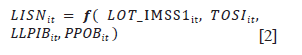
Where:
i = (1, ... , 32).
t = (2010, ... , 2020).
LISN it = natural logarithm of ISN for federal entity i during period t in pesos. The ISN is collected by employers based on labor transactions arising from employee service provision (Suprema Corte de Justicia de la Nación [SCJN], 2012; INEGI, 2022c).
LOT_IMSS1 it = natural logarithm of the number of workers registered with the Mexican Social Security Institute (IMSS) for federal entity i in period t, measured in thousands of workers. This variable quantifies the insured working population (those with a social security number in the institution) receiving medical services and economic benefits from this institution (IMSS, 2023; Tableau Software, 2022).
TOSI it = rate of occupation in the informal sector of federal entity i in period t. This measures the percentage of the employed population working in the informal sector (Banco de México [BANXICO], 2023; INEGI, 2022f).
LLPIB it = natural logarithm of the Gross Domestic Product (GDP) for federal entity i in period t, in billions of constant 2013 pesos. It is the sum of the market value of final goods and services generated within the national territory during a specific period (INEGI, 2022e; INEGI, 2023).
PPOB it = total population of federal entity i in period t, in millions of inhabitants. It is the number of individuals living in a geographical area and forming a five-year age group according to their gender (INEGI, 2022b; CONAPO, 2023). We obtained the total population figures from CONAPO data, which provides projections for the population of Mexico and its federal entities from 2016 to 2050. Utilizing these numbers and INEGI's five-year data, we supplemented the series for the years 2010 to 2015.
A positive and significant relationship is expected with all variables except the rate of employment in the informal sector in each federal entity.
Estimation of the Model for ISN
Next, we present the estimation of SF for each of the three random error distributions (semi-normal, exponential, and truncated normal). Subsequently, the distribution with the best fit is selected. In case of no consensus among the criteria, the distribution is chosen if at least 2 out of the 3 criteria consider it the best option.
Based on the findings presented in Table 3, the Wald statistic (2631.01) and BIC statistic (404.2219) both indicate that the semi-normal distribution demonstrates the strongest fit. Therefore, this error distribution model has been chosen for the analysis. The detailed estimates are provided in Annexes 1, 2, and 3.
Table 3 ISN Statistics
| STOCHASTIC FRONTIER | |||
|---|---|---|---|
| Random Errors Probability Distribution | Wald Statistic | Bayesian Information Criterion (BIC) | Log Likelihood |
| Semi normal | 2631.01 | 404.2219 | -181,58822 |
| Exponential | 2156.01 | 415.8714 | -187,41298 |
| Truncated normal | 2420.64 | 406.4381 | -179,76454 |
Source: Own elaboration.
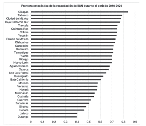
The SF is a model that assumes a tax collection function exposed to random shocks, with a degree of inefficiency in revenue collection that prevents federal entities from realizing their full potential. Thus, technical efficiency is within the range of (0, 1], where if it is equal to 1, tax collection would be entirely efficient, and if less than 1, it would be inefficient (Guillermo & Vargas, 2016). The estimation of average inefficiency in ISN collection processes is graphically presented below, with federal entities ordered from most to least efficient. In other words, the most efficient federal entity is the one closest to the value of 1.
Source: Own elaboration.
Figure 1 Average Estimated Inefficiency in ISN Tax Collection from 2010 to 2020
Chiapas is the entity with the highest efficiency in tax collection (0.8383), followed by Tabasco (0.7904), Mexico City (0.7769), Baja California Sur (0.7707), and Tlaxcala (0.7474). These results align with Guillermo and Vargas (2016), indicating that Chiapas, Mexico City, and Tlaxcala achieve the highest levels of revenue collection. Similarly, the satisfactory outcome observed in Mexico City coincides with Bonet and Rueda (2011), Puente and Rodríguez (2011) , and Castañeda and Pardinas (2012) . In contrast, Durango (0.3973) is the most inefficient state in the collection of ISN, followed by Jalisco (0.4014), Sonora (0.4607), Sinaloa (0.4784), and Zacatecas (0.5037). Guillermo and Vargas (2016) also agree that Jalisco is one of the entities with higher inefficiency in revenue collection. Table 4 presents the average efficiency value of ISN during the period 2010-2020 for each federal entity.
Table 4 Average Efficiency of ISN during the Period 2010-2020
| State | Efficiency |
|---|---|
| Chiapas | 0.838315791 |
| Tabasco | 0.790469645 |
| Ciudad de México | 0.776978318 |
| Baja California Sur | 0.770774482 |
| Tlaxcala | 0.747413064 |
| Quintana Roo | 0.746172227 |
| Colima | 0.744264118 |
| Yucatán | 0.741143991 |
| Estado de México | 0.731575745 |
| Chihuahua | 0.726720673 |
| Campeche | 0.7144832 |
| Querétaro | 0.7110215 |
| Tamaulipas | 0.710780773 |
| Puebla | 0.701345955 |
| Hidalgo | 0.6999605 |
| Nuevo León | 0.699190736 |
| Aguascalientes | 0.680545355 |
| Oaxaca | 0.673293436 |
| San Luis Potosí | 0.649586709 |
| Guanajuato | 0.625934655 |
| Baja California | 0.603386727 |
| Morelos | 0.5772102 |
| Veracruz | 0.574165318 |
| Nayarit | 0.572293127 |
| Michoacán | 0.550536627 |
| Coahuila | 0.544486 |
| Guerrero | 0.517252227 |
| Zacatecas | 0.503717991 |
| Sinaloa | 0.478437082 |
| Sonora | 0.460770145 |
| Jalisco | 0.401427655 |
| Durango | 0.397393782 |
Source: Own elaboration.
Specification of the Model for ISH
The function to estimate the MFE of the ISH is as follows:
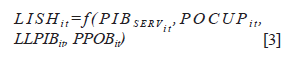
Where:
i = (1, .... , 32)
t = (2010, ... , 2020)
LISN it = natural logarithm ISH for federal entity i during period t in pesos. This variable measures the revenue from lodging services (DATATUR, 2023a). The hotelier is the withholder of this tax, while the guest is the one who pays this tax (DATATUR, 2023b; INEGI, 2022d).
PIB SERVit = percentage of the GDP generated in the temporary accommodation and food and beverage preparation sector of federal entity i in period t (DATATUR, 2023a). This variable encompasses the activities of temporary accommodation service companies (hotels, motels, cabins, and campsites, for example) along with the preparation and sale of food and beverages, both for on-site consumption and take-out (México ¿Cómo vamos?, 2023).
POCUP it = hotel occupancy rate percentage of federal entity i in period t (DATATURa). This counts the number of occupied rooms divided by the total available rooms during a specific period. It is then multiplied by 100 to express it as a percentage (DATATUR, 2023b).
LLPIB it = natural logarithm of the Gross Domestic Product (GDP) for federal entity i in period t, in billions of constant 2013 pesos. It is the sum of the value of final goods and services generated within the country's territory during a specific period (INEGI, 2023).
PPOB it = total population of federal entity i in period t, in millions of inhabitants. It is the number of individuals living in a geographical area and forming a five-year age group according to their gender (INEGI, 2022b; INEGI, 2022e; CONAPO, 2023). We obtained the total population figures from CONAPO data, which provides projections for the population of Mexico and its federal entities from 2016 to 2050. Utilizing these numbers and INEGI's five-year data, we supplemented the series for the years 2010 to 2015. A positive and significant relationship is expected with all variables.
While published works on estimating technical efficiency using this methodology have significantly increased in recent years, there is still no consensus on the best method for its estimation (Vergara, 2006). Therefore, to calculate the technical efficiency of the federal entities in collecting ISN and ISH, three probability distributions of random errors are evaluated: semi-normal, exponential, and truncated normal (Romero, 2016). In order to choose the probability distribution of random errors that provides the best fit, three criteria were employed: the Wald statistic, the Bayesian Information Criterion (BIC), and the log-likelihood (Fried et al., 2008). The objective of each of these criteria is detailed below, along with their decision rule.
The Wald statistic measures the overall significance of the estimated model. According to this criterion, the higher the value of the Wald statistic, the greater the evidence that the explanatory variables contribute to the variation of the dependent variable (Berger, 1997). On the other hand, the Bayesian Information Criterion (BIC) considers that the model with the best fit will be the one that minimizes this information criterion, i.e., the one with a lower BIC (Berger & Humphrey, 1997). Finally, according to the log-likelihood function, the most suitable model for describing the relationship between the variables under study-or the most likely in statistical terms is the one whose absolute value is greater (Berger & Humphrey, 1997). The 'FRONTIER' module of the STATA software (STATA, 2023) is utilized for estimating the SF function.
Estimation of the Model for ISH
Once again, the FRONTIER software is used. The results of the three statistics for each of the distributions of random errors are presented in Table 5. According to the results, both the Wald statistic (530.11) and the log-likelihood (-392.37429) indicate that the semi-normal distribution has the best goodness of fit. The detailed estimates are shown in Annexes 4, 5, and 6. The semi-normal error distribution is chosen because 2 out of 3 tests indicate it as the most appropriate. Annex 4 presents the estimated coefficients with a semi-normal distribution.
Table 5 ISH Statistics
| STOCHASTIC FRONTIER | |||
|---|---|---|---|
| Probability of Distribution in Random Errors | Wald Statistic | Bayesian Information Criterion (BIC) | Log Likelihood |
| Semi normal | 530.11 | 825.6736 | -392.37429 |
| Exponential | 506.19 | 823.3989 | -391.23692 |
| Truncated normal | 505.68 | 829.2469 | -391.23771 |
Source: Own elaboration.
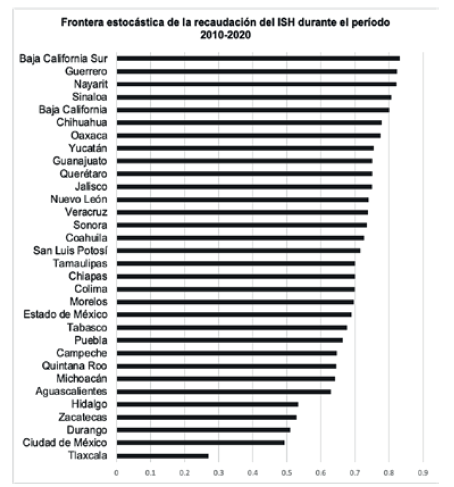
Next, Figure 2 illustrates estimation of average inefficiency in ISH collection processes, with federal entities ordered by their efficiency from highest to lowest. In other words, the most efficient federal entity is closer to the value of 1.
Baja California Sur is the federal entity that efficiently collects ISH (0.7752), followed by Guerrero (0.7613), Nayarit (0.7564), Sinaloa (0.7324), and Baja California (0.7248). It is interesting to contrast these results with the average collection of this tax per federal entity (Table 4). The nominal average hotel tax collection from 2010 to 2020, in descending order, is led by Baja California Sur ($211,654,190), Guerrero ($98,233,563), Nayarit ($114,749,642), Sinaloa ($72,168,053), and Baja California ($78,514,655). Thus, it is observed that there are entities that collect more money but are not necessarily the most efficient in their collection. This highlights that if there is an increase in productive activity, local governments need to have more efficient management and oversight capabilities to collect revenue. It is worth noting that Guillermo and Vargas (2016) observed the same during the 2003-2010 period.
Source: Own elaboration.
Figure 2 Average Estimated Inefficiency in ISH Tax Collection from 2010-2020
On the other hand, the least efficient entities in collecting ISH are Tlaxcala (0.2191), followed by Durango (0.3782), Mexico City (0.3811), Hidalgo (0.3983), and Zacatecas (0.3994). The average collection of the tax from 2010 to 2020 was: Tlaxcala ($2,012,465), Durango ($6,281,214), Mexico City ($320,900,365), Hidalgo ($8,181,185), and Zacatecas ($6,975,843).
Table 6 Average Efficiency of ISH during the Period 2010-2020
| State | Efficiency |
|---|---|
| Baja California Sur | 0.83267982 |
| Guerrero | 0.82336818 |
| Nayarit | 0.82116031 |
| Sinaloa | 0.80658847 |
| Baja California | 0.80095883 |
| Chihuahua | 0.77767357 |
| Oaxaca | 0.77567546 |
| Yucatán | 0.75402045 |
| Guanajuato | 0.75046216 |
| Querétaro | 0.75039113 |
| Jalisco | 0.74904973 |
| Nuevo León | 0.74059414 |
| Veracruz | 0.73746398 |
| Sonora | 0.73581344 |
| Coahuila | 0.72585432 |
| San Luis Potosí | 0.7160795 |
| Tamaulipas | 0.70044968 |
| Chiapas | 0.69977346 |
| Colima | 0.6996249 |
| Morelos | 0.69592659 |
| Estado de México | 0.6903314 |
| Tabasco | 0.67697228 |
| Puebla | 0.66445532 |
| Campeche | 0.64660547 |
| Quintana Roo | 0.64506105 |
| Michoacán | 0.64242421 |
| Aguascalientes | 0.62894697 |
| Hidalgo | 0.5341748 |
| Zacatecas | 0.52830313 |
| Durango | 0.51006159 |
| Ciudad de México | 0.49308113 |
| Tlaxcala | 0.27006362 |
Source: Own elaboration.
The MFE estimates for both ISN and ISH are conducted using a semi-normal distribution of random errors. Despite this commonality, the results obtained differ between the two taxes. In the stochastic collection frontier of ISN, the states are ranked as follows: Chiapas is the most efficient, followed by Tabasco, Mexico City, Baja California Sur, and Tlaxcala, based on payroll registration. On the other hand, the least efficient entities were Durango, Jalisco, Sonora, Sinaloa, and Zacatecas.
Regarding the ISH frontier, Baja California Sur is the most efficient entity, followed by Guerrero, Nayarit, Sinaloa, and Baja California. These states are recognized for capitalizing on their tourist areas and beaches. Conversely, the least efficient entity was Tlaxcala, followed by Mexico City, Durango, Zacatecas, and Hidalgo.
In the ISH analysis, it is observed that entities with beaches and tourist activities are the most efficient, while this does not apply to ISN, as the collection of this tax varies according to the fluctuation of employees registered in companies. Baja California stands out as the only efficient entity in collecting both taxes. In summary, it is concluded that there are federal entities that collect more money but are not efficient in their collection. Local governments have different capacities for management and oversight of revenue collection, highlighting a situation that requires attention.
DISCUSSION
The estimation of the ISN aligns with the findings of Puente and Rodríguez (2011) and Guillermo and Vargas (2016), particularly regarding the number of workers affiliated with the IMSS, GDP at the state level, and total population at the state level. This consistency reinforces the validity of these variables as determinants of ISN tax collection in Mexico.
However, the efficiency of ISN collection varies significantly across different Mexican states and is influenced by several factors. The disparities in revenue collection efficiency suggest that local governments possess varying capabilities to manage tax collection processes effectively. Interestingly, states with higher GDP on average do not necessarily exhibit higher efficiency in ISN collection. This observation implies that local economic conditions, such as the composition of the workforce and the prevalence of informal employment, play a crucial role in determining tax collection outcomes. Moreover, fluctuations in the number of employees registered with the IMSS can directly impact the efficiency of ISN collection, highlighting the dynamic nature of this revenue source.
Similarly, the ISH estimation is consistent with the results of Puente and Rodríguez (2011) and Guillermo and Vargas (2016) concerning the total population at the state level.
Additionally, the GDP generated in the temporary accommodation and food and beverage preparation sector at the state level, as well as the rate of hotel occupancy, shows a strong alignment with the findings of Puente and Rodríguez (2011).
The efficiency of ISH collection is also influenced by several key factors. States with beachfront locations and significant tourist attractions tend to demonstrate higher efficiency in ISH collection. This correlation is primarily due to the fact that tourism generates a larger taxable base for accommodation taxes, thereby enhancing revenue collection. Furthermore, the overall economic context of a state, including factors such as GDP and employment rates in the tourism sector, plays a critical role in determining ISH collection efficiency.
These findings underscore the importance of adopting a tailored approach to enhancing ISH collection efficiency at the local level. Local governments must consider the unique economic conditions and industry dynamics within their jurisdictions to optimize tax collection strategies.
CONCLUSIONS
This study examines the effectiveness of tax collection for ISN and ISH across 32 Mexican federal entities during 20102020. In both cases the estimations are conducted utilizing the SF model, a widely used tool in public finance research, considering a semi-normal random error distribution.
The analysis highlights disparities in revenue collection efficiency, indicating differences in the capabilities of local governments. For the ISN Chiapas is identified as the most efficient state, followed by Tabasco, Mexico City, Baja California Sur, and Tlaxcala. Conversely, Durango, Jalisco, Sonora, Sinaloa, and Zacatecas are noted as the least efficient in ISN collection. States that demonstrate the highest levels of efficiency do not necessarily correspond with those having the highest GDP or receiving the lowest intergovernmental transfers.
The analysis of the ISH presents a different scenario. Baja California Sur emerges as the most efficient entity, along with Guerrero, Nayarit, Sinaloa, and Baja California. It is interesting to note that entities with coastal areas and significant tourist attractions exhibit higher efficiency in ISH collection. Conversely, Tlaxcala, Mexico City, Durango, Zacatecas, and Hidalgo are identified as the least efficient in ISH collection.
The analysis conducted by ISH indicates that entities with beachfront locations and tourist attractions demonstrate higher levels of efficiency. In contrast, the ISN data shows that tax collection is subject to fluctuations based on changes in employee numbers. Baja California emerges as the sole entity demonstrating efficiency in both tax categories. We also found that states with higher revenue collection rates may not necessarily be the most efficient in their tax collection practices. The study underscores the importance of effective management and oversight capabilities, particularly considering fluctuations in employee registration for ISN and the dynamics of tourism for ISH.
These findings stress the importance of tailored approaches at the local level to improve revenue collection efficiency. Local governments must address specific challenges within their economic and social contexts, taking into consideration factors affecting tax collection for both ISN and ISH. This study offers valuable insights for policymakers, serving as a foundation for well-informed decision-making to enhance the fiscal environment in Mexican federal entities.

