


 English (pdf)
 Article in xml format
 Article references
 Send this article by e-mail
 Cited by SciELO
  Cited by Google
  Similars in
SciELO
Similars in
SciELO  Similars in Google
 Permalink
INTRODUCTION
Gold has historically been a better valued metal than silver, as well as being preferred by investors in times of crisis (Kumar et al., 2024). In recent years, however, silver has gained some notoriety for offering very competitive returns in relation to gold in addition to being much more accessible in terms of price. The question arises as to which of the two commodities is the better one to invest in. A review of the literature did not reveal any evidence that definitively answers this question. Also, no specific method was found that financially evaluates and compares the advantages and disadvantages of investing in one metal or the other. Therefore, the objective of this research was to determine which of the two metals is the best to invest in. Given the above, the main hypothesis was established: it is better to invest in gold than in silver1.
In order to respond to the research hypotheses, an empirical method was developed based on the five most common financial tests found in the literature (Bod'a & Kanderová, 2020; Gokmenoglu & Fazlollahi, 2015; Matiushin, 2019; Vacio, 2023; Zhang (2024), which were:
Financial integration with macroeconomic variables of the United States.
Predictability and Trend Analysis.
Loss rate.
Volatility analysis
Annual returns in the short, medium and long term.
In order to synthesize the results of the tests performed and to be able to determine which commodity is best to invest in, a decision making method based on the Pugh matrix was used (Okuyucu & Tanik, 2023).
Therefore, in the methodology stage a quantitative research approach was established, limited to the United States of America. The main variables included were: the price per ounce of gold and silver (USD) and its returns. The US macroeconomic variables added exclusively for the first test were: inflation; the price of crude oil (USD); the NASDAQ, S&P500 and Dow Jones indexes; the dollar exchange rate with the Great Britain pound (GBP/USD), the euro (EUR/USD) and the Chinese yuan (CNY/USD) were also included2.
For the timeline, what was observed by Iuorio (2023) and Sadorsky (2021) in the literature review was taken into account in relation to the crisis periods considered in modern history that affected the price of both metals. Therefore, the analysis period was limited from January 1990 to April 2024.
The information presented contributes to the literature in several specific ways, which were commented on in the results stage and as a synthesis in the conclusions. This research seeks to shed light on those individual investors, institutions and the public interested in buying gold and silver, but who have not yet decided which one to invest in. In the end, some considerations have been included that should be taken into account when investing in these metals.
LITERATURE REVIEW
Brief History of the Role of Gold and Silver in Finance
Since the appearance of the first tribal societies in the Neolithic (6000 B.C.), gold and silver began to be valued as important elements in ceremonial and cult themes, in the production of amulets and pieces related to divinity. It was not until 3000 B.C. that the Sumerians and Egyptians began melting down gold and silver to create luxury items, giving rise to what we know today as fine jewelry. The practice of using both metals in relation to magnificence and worship can also be found in the Torah or Pentateuch (the five books of Moses from exodus to Deuteronomy) which is believed to be written between 1300 B.C-1000 B.C., where gold is cited 143 times and silver another 87. The custom of using both metals for luxury and/or religious purposes has remained ever since.
On the financial topic, Kurke (2021) points out that according to the historian Herodotus, the first gold coins were minted by the kingdom of Lydia (present-day Turkey) between the year 650 B.C. and 490 B.C. This practice continued in subsequent civilizations until it arrived in the Americas in the 16th century. A couple of centuries later several countries began using a bimetallic standard (based on gold and silver) to back banknotes in circulation controlled by policy makers. In 1971, President Nixon released control over the price of gold set at $35 per ounce and in 1974 the United States Congress in turn removed the restriction on private holdings of gold (established since 1934) causing that the price of this metal will float in the coming years until stabilizing during the 80s.
In the following decades, Iuorio (2023) identified four stages of recession which impacted the price of gold and silver in modern history:
• 90s crisis
This crisis occurred in the early 90s, when the United States entered a mild recession promoted mainly by the increase in public debt carried over from the Ronald Reagan administration. The costs of the Cold War and low revenue (due to the reduction in the tax burden) took their toll. This mild recession resulted in a 16.13% decrease in the average price of gold (which was $350.99 per ounce during the 90s) compared to the average price of the previous decade (which was $418.49) (Investing 2024a). However, despite the drop in the average value of the metal, its price remained remarkably stable throughout most of the 1990s (Figure 1).
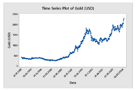
Source: Author's own elaboration, based on Investing (2024a), and Minitab software (2024).
Figure 1 Historical price of gold, from January 1990 to April 2024.
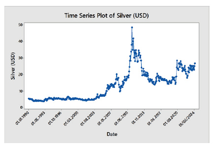
Source: Author's own elaboration, based on Investing (2024b), and Minitab software (2024).
Figure 2 Historical price of silver, from January 1990 to April 2024
Like gold, silver also presented a period of stability during the 90s (Figure 2). Neal and Weidenmier (2003) explained that this period of stability in both metals price was derived from the rise in the United States stock market which gave greater strength to the financial sector in those years.
• Second and Third Crisis (2000s)
It was not until the beginning of the 2000s that there was a significant increase in the price of both commodities, observable in figures 1 and 2. This leap in the prices of gold and silver was as a consequence of a second and third periods of recession in modern history.
The second recession corresponds to the economic slowdown in mid-2001. This crisis called the dot-com bubble originated on Wall Street was produced by new technology companies that had a presence on the stock market but did not have the physical infrastructure to support the operations required for e-commerce, basing their value only on speculative issues, a creative website, and the Internet fad. In order to alleviate the crisis caused by the collapse of stock markets, the Reserve Bank reduced interest rates to historic lows (Martin et al., 2022). The consequence of the above was that investors moved to safer and more profitable investment options, increasing the demand for gold and silver.
The third period of recession came years later, due to the mortgage crisis of October 2008. The effect of the mortgage crisis was further deepened following a modification to the national debt limit by the US government in 2011. This recession called the debt ceiling crisis is not specifically pointed out by Iuorio (2023) but according to Sadorsky (2021), this crisis also impacted the value of both metals, especially the price of silver. These record increases are also visible in figures 1 and 2.
• Pandemic Crisis (2020)
The 2020 pandemic crisis had a strong impact on financial markets all over the world, also affecting several sectors such as manufacturing industries, agriculture, transportation, tourism, and others. According to Ahmed and Sarkodie (2021), this recession led to greater instability in the prices of various commodities such as corn, oil, and natural gas, and also affected the value of most metals, including gold, silver, copper and steel. In addition, Raza et al. (2023) considered this period as a stage of greater instability in the price of gold and silver.
In relation to the aforementioned crises, in recent years various authors have tried to explain the influence of different factors on the variation in the price of these metals. Ahmed and Sarkodie (2021) support the theory that said volatility is due to supply and demand, contrary to what was expressed by Beretta and Peluso (2022) who maintain that these volatility changes are subject to speculative issues of financial markets rather than supply and demand; Martin et al. (2022) stated that the factors that affect the price of gold have been inflation and interest rates, while Kayal and Maheswaran (2021) pointed out that this volatility is more due to the fluctuation of the exchange rate for dollars in the country where they want to acquire said metals.
Although these different perspectives do not agree on the causality of the behavior of these commodities, in the particular case of gold, there is a consensus that this metal continues to be perceived as a safe haven to this day (Kumar et al., 2024).
Research Background
As observed in the previous section, gold has managed to build a solid reputation as a safe haven investment fund, especially in the economic crises that have occurred throughout history (Kumar et al., 2024). However, in recent years silver has captured the interest of investors around the world for two fundamental reasons: returns and price, raising the question of which of the two metals is best to invest in. After conducting a review of the literature, no evidence was found that answers this question conclusively. Nor was there a specific method found that financially evaluated and comparatively the benefits and shortcomings of investing in one or another metal. Therefore, the objective of this research was to determine which of the two metals is the best to invest in. Given the above, the main hypothesis was established:
H1: It is better to invest in gold than in silver.
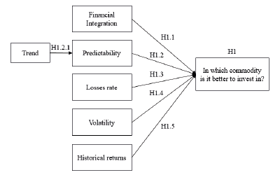
In order to respond to the main hypothesis, an empirical method was developed based on the five most common financial tests found in the literature, which were:
Financial Integration with Macroeco-nomic Variables of the United States
Given that gold and silver float freely depending on supply and demand, statistically comparing the price relationship of both commodities with macroeconomic variables of the United States (which in turn have a strong influence on the economy from all over the world), is relevant since it would allow us to infer which of the two metals has greater financial integration in relation to the degree of association they have with respect to the latter. Balcilar et al. (2020) commented that a strong financial integration between precious metals such as gold and silver, and macroeconomic variables, such as those of the United States stock market, inflation, oil prices, etc. would lead to greater exposure of these metals. It means that, if there is a financial crisis in these markets this would cause the price of these commodities to collapse, turning them into a viable investment option in the face of crises (transmuting them into safe havens). Farinha et al. (2020) say that the most common study to test such financial integration between this type of commodities and macroeconomic variables is correlation. In that sense, Zhang (2024) used the multiple linear correlation between the price of gold and some macroeconomic variables of the United States, such as S&P 500, EUR/USD exchange rate and the price of crude oil, finding a strong relationship between the price of gold and the latter.
In the present research, the scope of the study conducted by Zhang (2024) was extended to include the NASDAQ and Dow Jones indices, since according to Bacilar et al. (2020), these indices are an important indicator of the United States economy, which also have a strong impact on international financial markets. Also, other macroeconomic variables of the United States added were the exchange rates of the US dollar with the GBP, EUR and CYN which are currencies that also represent the economies with the most gold reserves (Forbes, 2024) and the that participate the most in the trade of this metal around the world (Statista, 2024). No evidence was found in the literature on the use of this test between the price of silver and the macroeconomic variables preceding. From the above, it was established:
H1.1: The price of gold has a stronger integration with macroeconomic variables of the United States than the price of silver.
Predi cta bility Analysis
A fairly common test used for decades to analyze the predictability of financial assets has been the ARIMA (Khalil, 2024). This tool has also seen its use expanded to project the price of various commodities effectively, including the price of gold (Bai, 2024; Khalil, 2024; Hong & Majid, 2021; Wang, 2023). Another tool used to analyze the volatility of the returns of financial instruments is the GARCH, which is an updated algorithm of the ARCH model that takes into account only the variance of the model errors but also the lagged variance, providing a more accurate model to capture the variation in returns of financial instruments that present certain volatility, such as gold (Bunnag, 2024; Madzar et al., 2023).
Furthermore, another arrangement used to a lesser extent for gold price prediction is Polynomial Regression (Kilimci, 2022; Vacio 2023). However, there is very little information on the use of the aforementioned methods in predicting the price of silver, which raises the question of which of the two commodities is easier to predict, based on the tools available in the literature, and how adept these are at predicting the future behavior of both metals. Likewise, another component related to the issue of predictability is knowing if the price of these metals has an upward trend over time. Both elements (predictability and trend) are important when considering investing in financial instruments. For this reason, it was defined:
H1.2: The price of gold is more predictable than that of silver.
H1.2.1: The price of gold has a greater upward trend than that of silver.
Loss Rate
Bod'a anf Kanderová (2020) proposed the use of Defects per Million Opportunities (DPMO) from the Six Sigma philosophy as a performance indicator on investment assets. This indicator is relevant, since it would show how frequent losses or drops would be expected in the returns of both metals with respect to time, complemented by the following analysis which would show how deep these losses are (volatility). The above would provide another perspective on the behavior of the volatility of both commodities mentioned by Ahmed and Sarkodie (2021), Beretta and Peluso (2022) and Kayal and Maheswaran (2021). No evidence of the use of DPMO in gold and silver was found. Therefore, it was stated:
H1.3: Gold has a lower return loss rate than silver.
Vo la tility Ana lysis
The literature abounds with information on the transmission of volatility between gold and silver (Koulis & Kyriakopoulos, 2023) and how gold volatility interacts with other markets (Kumar et al., 2023; Raza et al., 2023). Gokmenoglu and Fazlollahi (2015) carried out a volatility analysis using a variance test on the price of crude oil, gold and the S&P500 index and found similar volatility between all the study variables in the short term. As established by modern portfolio theory, a greater variation or volatility in the returns of an asset represents a greater investment risk (Zhou, 2022). No evidence was found specifically comparing volatility between gold and silver returns in the long term. Given the above, it was defined:
H1.4: Gold returns are less volatile than silver returns.
Annual Performance in the Short, Medium and Long Term
Matiushin (2019) conducted an analysis of the returns of gold and silver around the 2008 mortgage crisis, finding a significant difference in the returns of the two metals. In the present study, the time horizon used by Matiushin (2019) was extended considering the crisis periods observed by Iuorio (2023) in modern history, which had an impact on the price of both commodities from 1990 to 2024. Additionally, this timeline was segmented into three specific periods:
• Short term: from January 2020 to April 2024
According to Ahmed and Sarkodie (2021) and Raza et al. (2023), it was in those years when greater instability in the price of both metals could be seen. The above is derived from the 2020 pandemic crisis which strongly affected commodity markets around the world.
• Medium term: from January 2001 to April 2024
It was in this period that an upward trend occurred in the price of both commodities compared to other decades (figures 1 and 2). In addition, this period also includes several important crises, such as the one that occurred in the United States stock market in early 2000 called the dot-com crisis, the mortgage crisis of 2008 and the 2011 debt ceiling crisis, which had a major impact on gold and silver prices (Sadorsky, 2021).
• Long Term: from January 1990 to April 2024
This period includes the decade of the 90s, which according to Iuorio (2023), and Neal and Weidenmier (2003), it was characterized as a time-lapse of greater stability in the price of both metals. This period of stability is also observable in figures 1 and 2.
Segmenting the returns of both metals in the short, medium and long term would offer a broader perspective on the behavior of such returns in front of scenarios of crisis, prosperity, and stability in the economy. Therefore, it was defined:
H1.5: Gold has better annual returns than silver, in the short, medium and long term.
In order to synthesize and compare the results of the tests applied on both metals, and being able to answer the research hypotheses raised in Figure 3, an evaluation was carried out based on the decision-making method called Pugh Matrix (Okuyucu & Tanik, 2023), which allows comparing positive and negative aspects between two or more alternatives (gold and silver in this case), using as evaluation criteria the results of the financial tests.
The final result aims to shed light on those individual investors, institutions and the public who plan to buy gold and silver, but who have not yet decided in which of the two commodities to invest.
METODOLOGY
Since the objective of this research was to know which of the two metals, gold and silver, is the best to invest in, a quantitative research approach was established, limited to the United States for three main reasons:
To compare the degree of financial integration between the price of gold and silver with macroeconomic variables of the United States, which in turn have a strong link with the regional and global economy (Bacilar et al., 2020).
Because of the role that both commodities have played in the economy of that country throughout history and their impact on international markets.
Because the price per ounce of gold and silver is denominated in U.S. dollars (USD).
Therefore, for this research the following variables were included:
Gold price per ounce (USD) (GCQ4) (Investing, 2024a)
Silver price per ounce (USD) (SIN4) (Investing, 2024b)
Furthermore, in order to expand the study conducted by Zhang (2024), the following macroeconomic variables were included, exclusively for the first test (Financial Integration)3:
United States Inflation (U.S. Inflation Calculator, 2024)
Crude oil price (USD) (Macrotrends, 2024a)
NASDAQ Index (IXIC) (Investing, 2024c)
S&P500 Index (SPX) (Investing, 2024d)
Dow Jones Index (DJI) (Investing, 2024e)
Euro / Dollar exchange rate (EUR/ USD) (Investing, 2024f)
Great Britain Pound / Dollar exchangerate (GBP/USD) (Investing, 2024g)
Chinese Yuan / Dollar exchange rate (CNY/USD) (Macrotrends, 2024b)
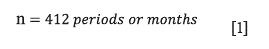
For the timeline, what was observed by Iuorio (2023) and Sadorsky (2021) was taken into account in the theoretical framework in relation to the crisis periods considered in modern history, which have had an important impact on the prices of both gold and silver. Therefore, the analysis period was limited from January 1990 to April 2024, obtaining for the study variables a total of:
In order to respond to the research hypothesis (Figure 3), the tests applied on the selected variables are shown below.
Financial Integration with Macroeconomic Variables of the US
Based on the analysis developed by Zhang (2024), a multiple linear correlation study was performed between the price of gold and silver and the macroeconomic variables considered in the present study. This method is expressed as follows (Montgomery & Runger, 2018):
The price of gold and silver is represented by y and the rest of the study variables by the control variables xt, x2, ..xn. In the end, the correlation indexes obtained showed the degrees of association that existed amid all the variables considered in the test arranged in the form of a matrix with the aim of answering H1.1.
Predictability and Trend Analysis
One of the most used tools when it comes to predicting the price of gold is ARIMA, which according to Bunnag (2024) is expressed by:
The elements that integrate the ARIMA model (p,d,q) are an autoregressive component (p), a moving average element (q), its coefficients ɸ and Ө and the number of lags applied to the series in case of correcting any unit root problem (d). In that sense, previously and with the objective of testing whether the series of both the price of gold and silver had the aforementioned characteristics, the Augmented Dickey-Fuller test was used, which is described as (Susanti et al., 2024):
In the case of t, this parameter represents the range between the values of the series (δ ̂) and the standard error of the same data (seδ ̂). By obtaining an H1: δ< 0 it would indicate that the series is stationary. Once the fact that both series had a random walk was verified, the data was converted into white noise using first differences technique, which has the following algorithm (Mohamed, 2020):
Once the ARIMA models were generated in both metals, a Box-LJung-Box test was performed to test the residuals stationarity of both arrangements. This test is expressed by (Mohamed, 2020):
Where r k is the autocorrelation of the data in a k period and m is the established number of lags. Subsequently, several clusters of variation in the errors of the ARIMA models were noticed, so to extend this observation an autoregression of the squared errors with one lag was performed. Then, an ARCH LM (Lagrange Multiplier) test was carried out, which is structured as follows (Susanti et al., 2024):
In the previous expression, R 2 is the coefficient of determination of the model, where a p-value <.05 in the test would imply that the data are not homoscedastic. Once the heteroske-dasticity of the squared residuals of the ARIMA models was corroborated, the GARCH models for gold and silver were assembled using the following algorithm (Bunnag, 2024):
The GARCH model is an extension of the ARCH model which not only considers the variance of the model errors, but also the lagged variance which has in its structure an AR component AR
 and an ARCH element
 .
.
Another of the prediction models used to predict financial instruments and commodities such as gold is polynomial regression, which according to Lee and Lee (2020) is expressed by:
With the objective of testing the significance of the polynomial models of order 1 to 6 built for both metals, an ANOVA test was executed using the F-test (Fisher) approach (Lee & Lee, 2020):
In which, the element SSLOP represents the sum of the lack of fit, SSPEI the sum of the squared errors, n the sample size, and p the number of terms in the model. A value of F > F α would indicate that the fit of the m-order regression model is significant.
Once the most common prediction tools on the gold price were developed (for both metals), their adjustability and relative quality were compared using the Akaike Information Criterion (AIC) and Bayesian Information Criterion (BIC), which are expressed in the following way (Mohamed, 2020):
In the case of BIC, this algorithm benefits from the relationship between simplicity and quality of fit relationship in the evaluated models as long as there is a sufficient sample size n, compared to the AIC criterion which will highlight the arrangement with the best possible fit without taking in consideration n or the complexity of the model according to its number of terms.
In the end, a table was prepared with the values obtained from the AIC and BIC of each tool included in this section with the objective of analyzing whether both metals have the characteristics of predictability, based on the adjustment capacity and relative quality that these models have and their ability to predict future values of both the price of both gold and silver and thus be able to respond to hypothesis H1.2.
In addition, some of the tests developed at this stage such as the Augmented Dickey-Fuller test (on gold and silver time series) the analysis of the coefficients and the R and R2 values (of the most significant polynomial models) helped to identify whether gold had a greater upward trend than that of silver and in turn to answer H1.2.1.
Loss Rate
Based on the proposal made by Bod'a and Kanderová (2020) and with the objective of obtaining the loss rate, the DPMO was estimated in both metals. One way to obtain this indicator is through a capacity study, which according to Montgomery and Runger (2018) is expressed by:
By using a Lower Specification Level (LSL) = 0, the model estimated the expected returns below zero (losses) per million events (months). By converting this indicator into a percentage, it gives us an estimate of the number of months per year in which losses are expected in both metals (H1.3).
The result of the capacity study performed by software Minitab (2024) was accompanied by an Anderson-Darling normality test, which according to Tapia and Cevallos (2021) is described by:
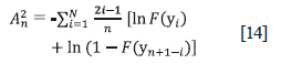
Where:
n = Sample size
y¡ = Ordered observations
F(y¡) = Distribution function
The results of the normality test were necessary for the next test.
Volatility Analysis
After performing a graphic analysis on both metals, it was observed that silver monthly returns presented greater volatility. To corroborate the above and based on the analysis developed by Gokmenoglu and Fazlollahi (2015), a variance difference test was run between both metals returns. Since the returns of gold and silver do not correspond to a normal distribution, the Bonett test was used for the difference in variances for two groups of non-normal data (Banga & Fox, 2013):
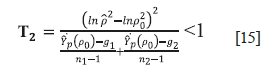
The hypothesis criterion used in this case was
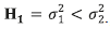 where
where
 is the variance of gold returns and
 the variance of silver returns. This model considers a parameter
 that represents a Pearson correlation coefficient of the standard deviation of the two groups of data, in this case the returns of both metals, where
 is given by
 .
The result would statistically confirm whether monthly gold returns are less volatile than silver returns (H1.4).
.
The result would statistically confirm whether monthly gold returns are less volatile than silver returns (H1.4).
Annual Performance in the Short, Medium and Long Term
To estimate the annual performance of both commodities, it was decided to extend the time period used by Matiushin (2019), seeking to include the economic crises that occurred in modern history contemplated by Iuorio (2023) and Sadorsky (2021) from 1990 to 2024. Furthermore, this timeline was segmented into three specific periods4 based on what was observed by Ahmed and Sarkodie (2021), Neal and Weidenmier (2003) and Raza et al. (2023):
Short term: from January 2020 to April 2024
Medium term: from January 2001 to April 2024
Long Term: from January 1990 to April 2024
The above allows us to have a broader perspective on the behavior of the returns of both metals, given the different scenarios of stability, prosperity and crisis in the economy. For each period, the average monthly performance was obtained using confidence intervals for the means, which according to Montgomery and Runger (2018), are given by:
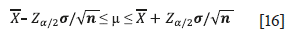
Where:
μ = Population mean
 = Sample mean
σ = Stanard deviation
 = Reference value on normal std. distribution
n = Sample size
Subsequently, for replying H.1.5 a table of results was constructed with the expected returns already annualized for each of these three scenarios proposed.
Evaluation Matrix
In order to synthesize of the test results and financially value the two commodities, a matrix was built based on a decision making method called Pugh analysis (Okuyucu & Tanik, 2023) which serve to compare several alternatives with each other based on evaluation criteria, that has the following structure:
Table 1 Evaluation Matrix Structure
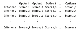
Source: Author's own elaboration, based on Okuyucu and Tanik (2023).
In this case, both metals represented the solution alternatives, and the tests performed represented the evaluation criteria. The scale used was consisten with the model proposed by Okuyucu and Tanik (2023): Plus (+1), Minus (-1), and Same (0) in relation to whether the evaluated alternative is better (+1), worse (-1) or similar (0) compared to the other alternative, according to the results of each test considered. The sum of the scores obtained determined which of the two commodities is the best to invest in (H1).
RESULTS
Financial Integration with Macroeconomic Variables of the US
In order to find out the relationship between the prices of both metals and the macroeconomic variables considered in this study, a multiple linear correlation analysis was executed.
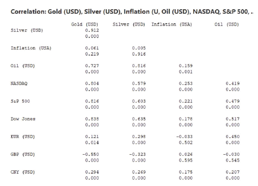
Source: Author´s own elaboration, based on Investing (2024a); Investing (2024b); U.S. Inflation Calculator (2024); Macrotrends (2024a); Investing (2024c); Investing (2024d); Investing (2024e); Investing (2024f); Investing (2024g); Macrotrends (2024b); and Minitab software (2024).
Figure 4 Multiple Linear Correlation
In Figure 4, it was confirmed that the price of gold has a close relationship with the price of a crude oil and the S&P500, which agreed with what was observed by Zhang (2024) in the period from December 2011 to December 2018. In addition, it was noticed that gold also has a strong relationship with the NASDAQ and Dow Jones indices. On the other hand, inflation, GBP, EUR and CYN exchange rates are not in sync with gold price.
It was also observed that the results for gold contrast with what was said by Farinha et al. (2020) who proposed that this metal is not linked to the stock market and cannot be considered as safe haven. However, the scope of the analysis carried out by the authors was from a short-term perspective based on the pre- and post-pandemic years (2019-2020). The present study took into consideration a broader period, considering the crises contemplated by Iuorio (2023) and Sadorsky (2021), from January 1990 to April 2024.
The above would add to the bibliographic heritage that the price of gold has a solid long term integration with the United States stock market. This qualifies it as a viable safe haven for those investments moving from high-risk stock market options into this metal with the aim of taking a long position.
In the case of silver, this metal cannot be considered for the same purpose.
Regarding silver, the present study would add to the literature that the price of this metal is also linked to the price of oil which would allow projections of the silver price based on this last commodity. Apart from this, no significant relationship was found between the price of this metal and the rest of the variables included in the analysis. Therefore, the price of gold has a better macroeconomic integration than that of silver (H1.1).
Predictability and Trend Analysis
A very common tool used in the literature to project the price of gold is the ARIMA (Bai, 2024; Khalil, 2024; Hong & Majid, 2021; Wang, 2023).
When analyzing the behavior of the historical series of both metals, contrary to the considerations required by the ARIMA model to be able to operate, they do not visually comply with the characteristics of zero mean and constant variance (Bunnag, 2024). To corroborate the above and based on the test suggested by Susanti et al. (2024), an Augmented Dickey-Fuller test was executed confirming the absence of stationarity (Figure 5).
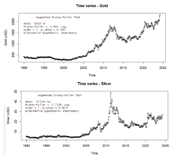
Source: Author's own elaboration, based on Investing (2024a), Investing (2024b), and RStudio Software (2024).
Figure 5 Gold and silver price series and Augmented Dickey-Fuller test.
Subsequently, both series were adjusted using the first-difference method (Mohammed, 2020). By re-running the Augmented Dickey-Fuller test, it was possible to confirm the stationarity of the returns of both commodities with a first-order differentiation, an adjustment that was sufficient like that carried out by Khalil (2024) and Bai (2024) to transform a time series of the gold price into white noise, also with the purpose of generating an ARIMA model to make projections.
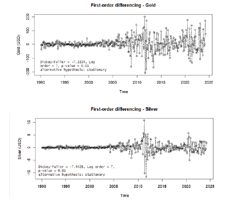
Source: Author's own elaboration with RStudio Software (2024).
Figure 6 First difference adjustment and second Augmented Dickey-Fuller test
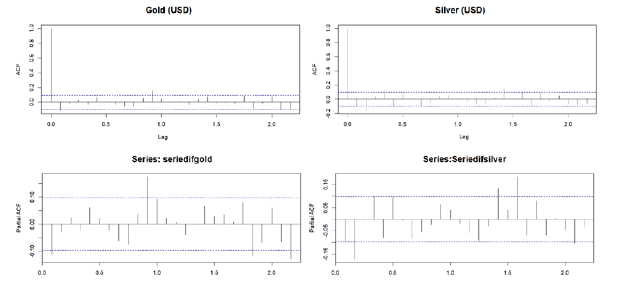
Source: Author's own elaboration with RStudio Software (2024).
Figure 7 Partial autocorrelation (PACF) and autocorrelation (ACF) components
Once the issue of stationarity was resolved, in Figure 7 a review of the partial autocorrelation (PACF) and moving average (ACF) components was performed observing 4 and 5 lags (PACF and ACF) in the case of gold, and 5-5 lags (also PACF and ACF) in the case of Silver. Bai (2024), Khalil (2024) and Wang (2023) found a much smaller number of lags in such components in the construction of their ARIMA models for gold projection. However, this is because the present study comprises a greater breadth of the sample size which covers a higher number of crisis periods contemplated by Iuorio (2023) from 1990 to 2024. With this information, ARIMA models were built for both metals.
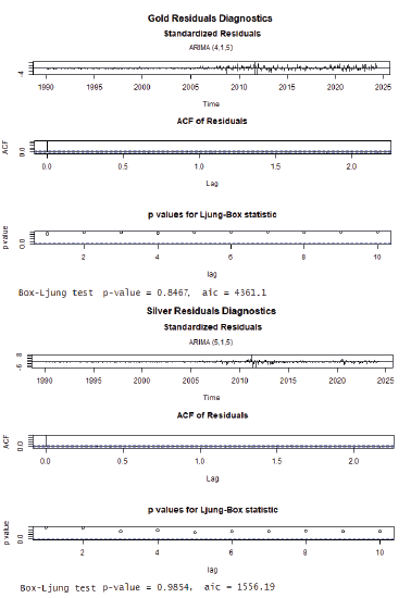
Source: Author's own elaboration with RStudio Software (2024).
Figure 8 Residual analysis and LJung-Box test in ARIMA models.
Once the ARIMA arrays were constructed, an analysis of the residuals in Figure 8 was performed to validate such models (Mohamed, 2020). The LJung-Box test yielded a p-value >.05, specifying that the errors of the ARIMA models for both gold and silver have the characteristic of white noise (stationarity). Besides, an AIC of 4361 was observed in the case of gold, similar to that estimated by Hong and Majid (2021) for an ARIMA model for the price of gold also. In relation to silver, the proposed ARIMA obtained an AIC of 1156. However, although the LJung-Box criterion confirms the validity of the proposed ARIMA algorithms, a slight variation in the models residuals is still observed. To expand this perspective, an analysis of the squared residuals was executed:
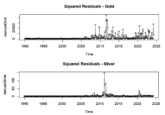
Source: Author's own elaboration with RStudio Software (2024).
Figure 9 Squared residuals analysis in ARIMA models.
In Figure 9, clusters of variation or heteroskedasticity can be spotted in periods that correspond to the 2008 mortgage crisis (Iuorio, 2023), the 2011 debt ceiling crisis (Sadorsky, 2021), and the 2020 pandemic crisis (Ahmed & Sarkodie, 2021; Raza et al., 2023). Starting from the principle of conditional variance (Bunnag, 2024), an autoregression of the squared errors with one lag was performed with the objective of testing whether the variation of the residuals in both models complies with the structure of an ARCH model.
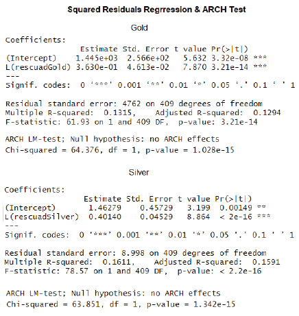
Source: Author's own elaboration with RStudio Software (2024).
Figure 10 Regression analysis of squared residuals and ARCH Test.
In the analysis of Figure 10, it was observed that the coefficients of the squared residuals with one lag are significant in both cases (t-value> 2). Also, the ARCH test advised by Susanti et al. (2024) revealed that the squared errors of the ARIMA models for Gold and Silver have heteroscedasticity under the premise of conditioned variance (p-value<.05). Bunnag (2024) and Kumar et al. (2024) also found the use of one lag in their GARCH models was enough to project gold and oil price volatility. Considering the above, the following first-order GARCH models were generated:
Source: Author's own elaboration with RStudio Software (2024).
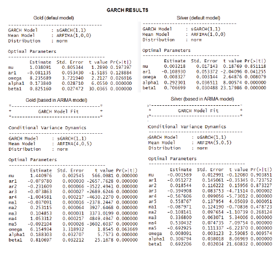
Figure 11 GARCH models and their coefficients.
To have a broader perspective, the GARCH (1,1) with ARFIMA (1,0,0) models were first obtained for both metals which are generated by default by the RStudio (2024) software. In this first iteration, the components that were not significant in both the gold and silver algorithms were the intercept (mu) and the autoregressive coefficient (ar1).
Regarding the constant of the GARCH model (omega), the coefficient of the variance with one lag (beta 1) and the coefficient of the squared residuals (alpha1), these turned out to have a significant effect in both arrangements. Subsequently, the GARCH models were generated based on the previous ARIMA models5 finding significance in several autoregressive and moving average coefficients and the intercept and the coefficients alpha1 and omega in the case of gold, and in omega, alpha1 and beta1 in the case of silver.
Another tool used by other authors to predict the behavior of gold is polynomial regression (Kilimci, 2022; Vacio, 2023). To find out the predictability of gold and silver prices using this tool, polynomial regression models from order one to six were generated:
Source: Author's own elaboration with RStudio Software (2024).
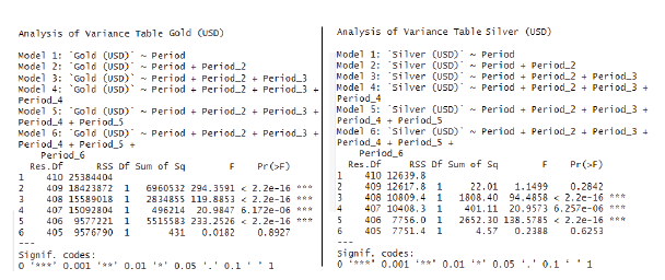
Figure 12 Polynomial regression models ANOVA.
Thereafter, the degree of significance of the models was evaluated using Analysis of Variance (ANOVA). Observing that, in the case of gold the 2nd, 3rd, 4th and 5th order models presented significant effects. On the other hand, in the case of silver only the 3rd, 4th and 5th term models exhibited a significant effect in the analysis. In both cases, including a 6th term they failed to improve their fit. The above contrasts with what was commented by Fahrudin et al. (2020) on who found a better fit in the 6th order model for predicting the price of gold based on a time-lapse between 2018-2020. Afterwards, an analysis of the coefficients was accomplished only in those models that presented a significant effect in the ANOVA.
Source: Author's own elaboration with RStudio Software (2024).
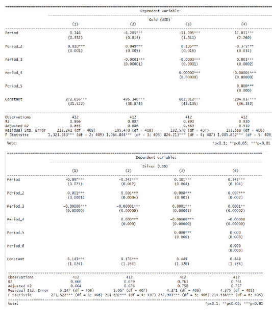
Figure 13 Analysis of the coefficients of the polynomial regression models.
When reviewing the coefficients of the most relevant polynomial algorithms, it was observed that in the case of gold, all the coefficients (and the intercept) of power 3, 4 and 5 (models 2, 3 and 4 in Figure 13) presented important significance (p< 0.01). The above is consistent with what was said by Vacio (2023), who found the order 3 model as the one that presents a better fit in the projection of gold.
As for silver, it was only the order 3 model (2 in Figure 13) that showed significant effects in all its terms. In the case of the power 4 algorithm, it was relevant in most of its coefficients, except for the intercept. Although this constant only represents a cut-off point in this last model, raising this arrangement one term (from order 3 to order 4) does not show a significant improvement in the matter of the residuals standard error (nor in the case of R2). Therefore, it can be stated that these two polynomial regression models are efficient to perform projections in the case of silver.
Table 2 Summary of the Prediction Models Performance
| Model | R2 | R2 Adjusted | Residual Std. Error | AIC | BIC | |
|---|---|---|---|---|---|---|
| Gold | ARIMA | - | - | - | 4361.10 | 4401.28 |
| GARCH (1,0), ARFMA (1,0,0) (Default model) | - | - | - | 9.72 | 9.76 | |
| GARCH (1,0), ARFMA (4,0,5) (Based in previous ARIMA)) | - | - | - | 9.70 | 9.82 | |
| 3rd Order Polynomial Regression | 0.887 | 0.886 | 195.470 | 5522.12 | 5542.23 | |
| 4th Order Polynomial Regression | 0.890 | 0.889 | 192.570 | 5510.79 | 5534.92 | |
| 5th Order Polynomial Regression | 0.930 | 0.930 | 153.588 | 5325.40 | 5353.55 | |
| Silver | ARIMA | - | - | - | 1556.20 | 1600.40 |
| GARCH (1,0), ARFMA (1,0,0) (Default model) | - | - | - | 2.46 | 2.50 | |
| GARCH (1,0), ARFMA (5,0,5) (Based in previous ARIMA)) | - | - | - | 2.47 | 2.61 | |
| 3rd Order Polynomial Regression | 0.679 | 0.676 | 4.371 | 2525.27 | 2545.38 | |
| 4th Order Polynomial Regression | 0.761 | 0.758 | 4.375 | 2511.69 | 2535.82 |
Source: Author's own elaboration.
Making a summary of the performance of the prediction models developed in this research, and taking into consideration the AIC and BIC values (Mohamed, 2020), those models that presented a better fit for the prediction of gold and silver were the GARCH arrays followed by the ARIMA algorithms, which obtained a similar criteria performance to those obtained by Gohs (2022) and Setyowibowo et al. (2022) in their ARIMA and GARCH models for gold.
Although polynomial regressions have less empirical support in terms of comparison criteria, these algorithms perform well in terms of the significance of the coefficients and their R and R2 values. The above would add to the literature the validity of the use of polynomial regressions as long as they are considered as secondary or complementary tests of other prediction models of greater robustness and in those cases where they look to test upward or downward trends over the long term.
Derived from the results of this section, it can be stated that both commodities have the characteristic of predictability based on the adaptability and relative quality of the developed models and their ability to predict future price values of the two metals, giving an answer to H1.2.
Likewise, the Augmented Dickey-Fuller test carried out on the time series of gold and silver (Figure 5) as well as the relevance of the coefficients and the R and R2 values obtained by the most significant polynomial models (Figure 13), confirm an upward trend for both commodities responding to H1.2.1.
Loss Rate
Subsequently, a capacity study of the monthly returns of gold and silver was conducted with the purpose of obtaining the DPMO for each commodity and, consequently, being able to determine the loss rate.
Source: Author's own elaboration, based on Investing (2024a), and Minitab software (2024).
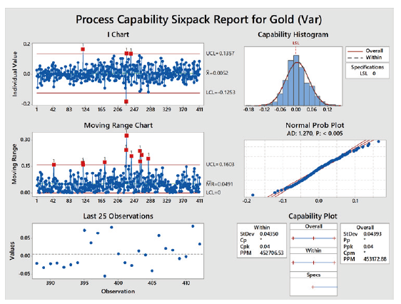
Figure 14 Capacity study on gold monthly returns, from January 1990 to April 2024
The capacity study graphically showed those months when returns were less than zero (losses) (Figure 14). According to the DPMO (PPMI or Parts Per Million in software), gold showed losses 45.27% of the time, that is in 5.43 months per year similar to the behavior observed by Siegel (2021) on gold returns in the long run. In the case of silver (Figure 8), the DPMO indicated that this metal would have a drop in returns 46.34% of the time, that is at approximately 5.56 months each year.
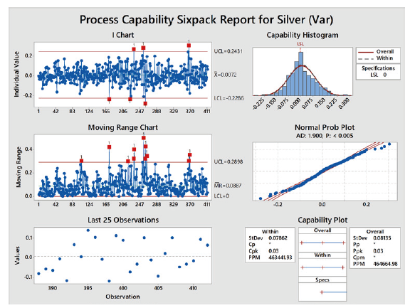
Source: Author's own elaboration, based on Investing (2024b), and Minitab software (2024).
Figure 15 Capacity study on silver monthly returns, from January 1990 to April 2024.
Based on the proposal of Bod'a and Kanderová (2020), it can be observed that both gold and silver exhibited a similar loss rate (H1.3). Although both commodities are expected to present losses for half of the year, according to Xu (2024) these losses may occur due to several factors such as international conflicts as the war in Ukraine, the international monetary policy, interest rates, as well as changes in supply and demand by industries that require these metals as raw materials, such as jewelry, the manufacturing of electrical and electronic products, the automotive industry, etc.
Another result observed in figures 14 and 15 was the Anderson-Darling (AD) normality test, which indicated that the returns of both gold and silver did not follow a normal distribution. This result was required in the following analysis.
Volatility Analysis
When analyzing gold and silver returns graphically, they displayed the following behavior:
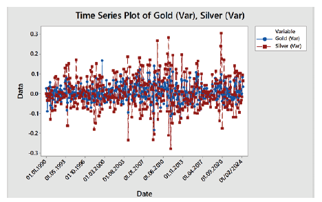
Source: Author's own elaboration, based on Investing (2024a); Investing (2024b); and Minitab software (2024).
Figure 16 Gold and Silver Returns per Month, from January 1990 to April 2024.
According to Figure 16, both metals experienced some volatility or variation in their historical returns. However, in the case of silver a deeper variation is seen especially throughout the 90's, 2004, 2008, 2011 and 2020, which agrees with the aforementioned periods of economic crashes (Ahmed & Sarkodie, 2021; Iuorio, 2023; Neal & Weidenmier, 2003; Raza et al. 2023; Sadorsky, 2021). To corroborate this difference in volatility, a variance difference test for non-normal data was performed.
The graph above indicates a greater amplitude in the variability of silver performance. Furthermore, the Bonett test showed with 95% reliability that the return of gold is less volatile with respect to the return of silver (P-value= 0). This point agrees with what was observed by Kayal and Maheswaran (2021) in a medium-term period from January 2001 to December 2016. Based on the test results and according to the modern portfolio theory explained by Zhou (2022), gold is the least risky commodity to invest in (H1.4).
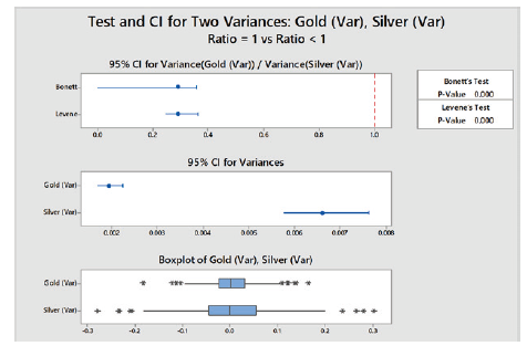
Source: Author's own elaboration, based on Investing (2024a); Investing (2024b); and Minitab software (2024).
Figure 17 Hypothesis test for the difference of variances, assuming non-normal data, under the criterion: Hi= Gold returns < Silver returns
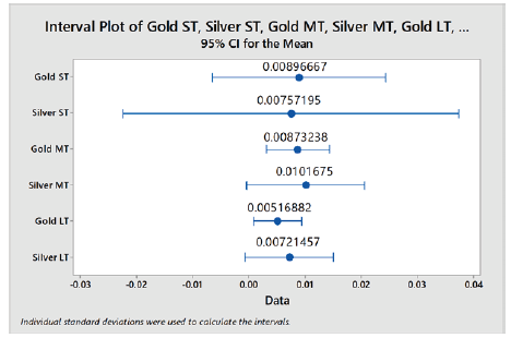
Source: Author's own elaboration, based on Investing (2024a); Investing (2024b); and Minitab software (2024).
Figure 18 Gold and silver average monthly returns segmented by short (ST), medium (MT) and long (LT) terms.
Annual Performance in the Short, Medium and Long Term
The average monthly returns were then estimated for the three time periods considered in this research, using confidence intervals for the means: With the previous information (Figure 18) it was possible to calculate the annual performance of each period, which can be seen in Table 3.
Table 3 Gold and Silver Annual Returns in Different Timeframes.
| Annual Returns | Short Term (January 2020 to April 2024) | Medium Term (January 2001 to April 2024) | Long Term (January 1990 to April 2024) |
|---|---|---|---|
| Gold | 10.7600% | 10.4789% | 6.2026% |
| Silver | 9.0863% | 12.2010% | 8.6575% |
Source: Author´s own elaboration, based on Investing (2024a) and Investing (2024b).
Regarding the results of Table 3, the annual return of gold stands out in the short term, which is consistent with the comments of Bai and Ho (2023), who observed a favorable behavior of gold returns despite the negative effect that the health crisis had on other commodities and financial assets around the world after 2020. In the case of silver, a higher annual return than that of gold was also observed in the medium and long term (H.1.5). According to Sadorsky (2021) and Xu (2024), the cause of this increase was due in part to the increase in debt contracted by the United States and several European countries in 2011, accompanied by a fall in interest rates which caused a notable peak in demand for this metal.
Evaluation Matrix
In order to synthesize the results of the tests and to be able to assess which of the two commodities is best to invest in, an evaluation matrix was developed based on the Pugh analysis (Okuyucu & Tanik, 2023):
Table 4 Evaluation Matrix Results
| Analysis Topics | Gold | Silver |
|---|---|---|
| Related to U.S. Stock Market | Yes (+1) | No (-1) |
| (NASDAQ, SP&500 & Dow Jones) | ||
| Related to Crude Oil Prices | Yes (0) | Yes (0) |
| Related to Yuan (USD), | Non (0) | Non (0) |
| EUR (USD) & GBP (USD) | ||
| Predictability | Yes (0) | Yes (0) |
| Long-Term Bullish Behavior | Yes (0) | Yes (0) |
| Loss rate | High(0) | High (0) |
| Volatile (Risk) | Less | More |
| (+1) | (-1) | |
| Short Term Returns | Better | Worse |
| (+1) | (-1) | |
| Medium Term Returns | Worse | Better |
| (-1) | (+1) | |
| Long Term Returns | Worse | Better |
| (-1) | (+1) | |
| (+) summation | +3 | +2 |
| (-) summation | - 2 | -3 |
| Final Score | 1 | -1 |
Source: Author's own elaboration, based on Investing (2024a) and Investing (2024b).
According to the result of the evaluation matrix (Table 4), it was observed that gold obtained a score of +1 while silver reached a value of -1. Therefore, according to the financial tests that conformed the empirical method developed in this research, gold is the metal in which it is most convenient to invest.
CONCLUSIONS
The results of this study contribute to the literature in four essential points:
1. The price of gold has a solid long-term integration with the U S stock market, but not with the foreign exchange market (EUR, GBP. or CYN). This qualifies it as an excellent safe haven when a shock hits the market for those investments that move from high-risk stocks to this metal. In the case of silver, it cannot be used for the same purpose. Therefore, in times of crisis silver positions would have to be moved to other types of investments options such as gold or government bonds.
2. While it is likely that the monthly returns of both metals will show losses for nearly six months of the year, it is also expected that such losses will be deeper or more violent for silver over time.
Due to the aforementioned volatility, forecasting tools such as GARCH and ARIMA can also be used, which have been successfully performed by other authors to predict gold (Bunnag, 2024; Gohs, 2022; Kumar et al., 2024; Setyowibowo et al., 2022), which in the present research showed a good quality of fit to predict the future behavior of both commodities and reduce uncertainty when investing. Furthermore, in the case of the price of silver, it showed a strong relationship with the price of oil, which can serve as a predictor variable on multivariate projection tools.
3. The present study has also shown the validity of using of polynomial regressions to forecast the price of gold and silver as a complementary test to other more robust forecasting models (such as ARIMA or GARCH), and in those cases it seeks to test long-term trends.
4. - Observing the results of the tests carried out it can be stated that gold is a less risky refuge fund with better returns in recent years, making it more viable to invest in the long term (bearish position) leaving silver as an asset more oriented to speculation (bullish position).
In the end, it was concluded that amid gold and silver, gold is the best commodity to invest in. However, there are some considerations to take into account when deciding to buy these metals:
• Supply and Demand:
Ahmed and Sarkodie (2021) commented that volatility in gold and silver prices is derived from changes in supply and demand, arguing that in recent years the electronics and manufacturing industry as well as the jewelry sector have seen a significant rise in demanding these metals as raw materials. Regarding the supply of gold, the production of this commodity has remained unchanged since 2016 (Statista, 2023) limiting the supply of this metal.
• Black Swan Events:
Events such as international conflicts, historic market shocks or pandemics could deeply impact on the prices of both commodities (Kumar et al., 2024). According to Xu (2024), the war in Ukraine and the increase in the price of oil impacted the volatility of gold and silver in the post-pandemic period.
• Exchange Rate to Dollars:
This aspect is relevant because the price of both commodities has two essential components: their market value (in USD) and the dollar exchange rate in the country where you wish to acquire these metals. This means that the fluctuation of the dollar exchange rate can create opportunities for trading these metals in those countries with different currencies than the USD (Kayal & Maheswaran, 2021).
• Historical Gold and Silver Returns vs Interest Rates:
It is important to observe the estimate of the annual returns of gold and silver in the short, medium and long term considered in this research, in comparison with the interest rates in the country where you wish to acquire these commodities (Beretta & Peluso, 2022; Martin et al., 2022),
• Regulatory and Fiscal Standards:
Besides, it is important to take a look at the tax and regulatory policies for trading and holding of precious metals in the area where you plan to invest in these commodities. As commented by Sugirtha and Manivannan (2018) in the case of India, where there was greater volatility in the prices of gold and silver prices due to the introduction of new tax rates on the trade of these metals.
The information provided in this research contributes to the extant literature on the aforementioned elements. It seeks to shed light on individual investors, institutions, and the public interested in acquiring gold or silver but haven't decided which is more convenient for their interests.

