1. Introduction

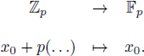
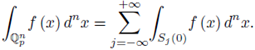
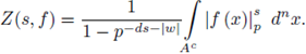
In these notes we provide an introduction to the theory of local zeta functions from scratch. We assume essentially a basic knowledge of algebra, metric spaces and basic analysis, mainly measure theory. Let be a local field, for instance the field of p-adic numbers, or the field of formal Laurent series with coefficients in a finite field with p elements. Let be a non-constant polynomial and let 92 be a test function. The local zeta function attached to the pair (h, 9) is defined as

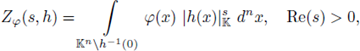
where denotes the absolute value of , s ∈ C, and d ⁿ x denotes a normalized Haar measure of the topological group ( ⁿ, +). These integrals give rise to holomorphic functions of s in the half-plane Re(s) > 0. If has characteristic zero, then admits a meromorphic continuation to the whole complex plane. The p-adic local zeta functions (also called Igusa's local zeta functions) are connected with the number of solutions of polynomial congruences mod p^m and with exponential sums mod p^m (see e.g., ^[14], ^[28], ^[31]).

In the Archimedean case, the study of local zeta functions was initiated by Gel'fand and Shilov ^21]. The meromorphic continuation of the local zeta functions was established, independently, by Atiyah ^[4] and Bernstein ^[6] (see also [31, Theorem 5.5.1 and Corollary 5.5.1]). The main motivation was that the meromorphic continuation of Archimedean local zeta functions implies the existence of fundamental solutions (i.e. Green functions) for differential operators with constant coefficients. It is important to mention here, that in the p-adic framework, the existence of fundamental solutions for pseudo differential operators is also a consequence of the fact that the Igusa local zeta functions admit a meromorphic continuation (see [33, Chapter 10] and [62, Chapter 5]).

On the other hand, in the middle 60s, Weil initiated the study of local zeta functions, in the Archimedean and non-Archimedean settings, in connection with the Poisson-Siegel formula ^[59]. In the 70s, Igusa developed a uniform theory for local zeta functions over local fields of characteristic zero ^[28], ^[30]. More recently, Denef and Loeser introduced in ^[15] the topological zeta functions, and in ^[16] they introduce the motivic zeta functions, which constitute a vast generalization of the p-adic local zeta functions.

In the last thirty-five years there has been a strong interest on p-adic models of quantum field theory, which is motivated by the fact that these models are exactly solvable. There is a large list of p-adic type Feynman and string amplitudes that are related with local zeta functions of Igusa-type, and it is interesting to mention that it seems that the mathematical community working on local zeta functions is not aware of this fact (see e.g. ^[2], ^[5], ^[7], ^[10]-[13], ^[18]-[20], ^[22]-[24], ^[27], ^[38], ^[39], ^[42], ^[48]-[52], and the references therein).

The connections between Feynman amplitudes and local zeta functions are very old and deep. Let us mention that the works of Speer ^[50] and Bollini, Giambiagi and González Domínguez ^[11] on regularization of Feynman amplitudes in quantum field theory are based on the analytic continuation of distributions attached to complex powers of polynomial functions in the sense of Gel'fand and Shilov ^[21] (see also ^[5], ^[7], ^[10] and ^[42], among others). This analogy turns out to be very important in the rigorous construction of quantum scalar fields in the p-adic setting (see ^[43] and the references therein).

The local zeta functions are also deeply connected with p-adic string amplitudes. In ^[8], the authors proved that the p-adic Koba-Nielsen type string amplitudes are bona fide integrals. They attached to these amplitudes Igusa-type integrals depending on several complex parameters and show that these integrals admit meromorphic continuations as rational functions. Then they used these functions to regularize the Koba-Nielsen amplitudes. In ^[9], the authors discussed the limit p approaches to one of tree-level p-adic open string amplitudes and its connections with the topological zeta functions. There is empirical evidence that p-adic strings are related to the ordinary strings in the limit p → 1. Denef and Loeser established that the limit p → 1 of a Igusa's local zeta function gives rise to an object called topological zeta function. By using Denef-Loeser's theory of topological zeta functions, it is showed in ^[9] that limit p → 1 of tree-level p-adic string amplitudes give rise to certain amplitudes, that we have named Denef-Loeser string amplitudes.

Finally, we want to mention about the remarkable connection between local zeta functions and algebraic statistics (see ^[40], ^[58]). In ^[58] is presented an interesting connection with machine learning.

This survey article is based on well-known references, mainly Igusa's book ^[31]. The work is organized as follows. In Section 2, we introduce the field of p-adic numbers, and we devote Section 3 to the integration theory over Section 4 is dedicated to the implicit function theorems on the p-adic field. In Section 5, we introduce the simplest type of local zeta function and show its connection with number of solutions of polynomial congruences mod p^m. In Section 6, we introduce the stationary phase formula and use it to establish the rationality of local zeta functions for several type of polynomials. Finally, in Section 7, we state Hironaka's resolution of singularities theorem, and we use it to prove the rationality of the simplest type of local zeta functions in Section 8.

For an introduction to p-adic analysis the reader may consult ^[1], ^[25], ^[32], ^[35], ^[46], ^[47], ^[53] and ^[56]. For an in-depth discussion of the classical aspects of the local zeta functions, we recommend ^[3], ^[14], ^[21], ^[28], ^[30], ^[31], ^[41]. There are many excellent surveys about local zeta functions and their generalizations. For an introduction to Igusa's zeta function, topological zeta functions and motivic integration we refer the reader to ^[14], ^[16], ^[17], ^[44], ^[45], ^[55]. A good introduction to local zeta functions for pre-homogeneous vector spaces can be found in ^[30], ^[31] and ^[34]. Some general references for differential equations over non-Archimedean fields are ^[1], ^[33], ^[56], ^[62]. Finally, the reader interested in the relations between p-adic analysis and mathematical physics may enjoy ^[12], ^[13], ^[19], ^[20], ^{[22]- [24]}, ^[27], ^[33], ^{[37]- [39]}, ^[43], ^[48], ^[49], ^[52], ^[54], ^[56], ^[57] and ^[62].

2. p-adic Numbers- Essential Facts

2.1. Basic Facts

In this section we summarize the basic aspects of the field of p-adic numbers, for an in-depth discussion the reader may consult ^[1], ^[25], ^[32], ^[35], ^[46], ^[47], ^[53] and ^[56].

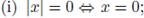
Definition 2.1. Let F be a field. An absolute value on F is a real-valued function, | · |, satisfying

Definition 2.2. An absolute value | · | is called non-Archimedean (or ultrametric), if it satisfies

Example 2.3. The trivial absolute value is defined as

From now on we will work only with non trivial absolute values.

Definition 2.4. Given two absolute values | · |₁, | · |₂ defined on F, we say that they are equivalent, if there exists a positive constant c such that

for any x ∈ F.

Definition 2.5. Let p be a fixed prime number, and let x be a nonzero rational number. Then, for some a ,b, k ∈ with p ∤ ab. The p-adic absolute value of x is defined as

Lemma 2.6. The function | · |_p is a non-Archimedean absolute value on

The proof is left to the reader. In fact, we kindly invite the reader to prove all the results labeled as Lemmas in these notes.

Theorem 2.7 (Ostrowski, ^[35]). Any non trivial absolute value on is equivalent to | · |_p or to the standard absolute value | · |_∞.

An absolute value | · | on F allow us to define a distance d(x, y) := |x − y|, x, y ∈ F. We now introduce a topology on F by giving a basis of open sets consisting of the open balls B _r (a) with center a and radius r > 0:

A sequence of points is called Cauchy if

A field F with a non trivial absolute value | · | is said to be complete if any Cauchy sequence has a limit point x* ∈ F, i.e. if |x_n - x*| → 0, n → ∞. This is equivalent to the fact that (F, d) , with d(x, y) = | x - y| , is a complete metric space.

Remark 2.8. Let (X, d), (Y, D) be two metric spaces. A bijection p : X → Y satisfying

is called an isometry.

The following fact is well-known (see e.g. ^[36]).

Theorem 2.9. Let (M, d) be a metric space. There exists a complete metric space such that M is isometric to a dense subset of

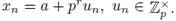
The field of p-adic numbers _p is defined as the completion of with respect to the distance induced by | · |_p. Any p-adic number x ≠ 0 has a unique representation of the form

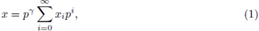
where The integer γ is called the p-adic order of x, and it will be denoted as ord(x). By definition ord(0) = +∞.

Lemma 2.10. Let (F, | · |) be a valued field, where | · | is a non-Archimedean absolute value. Assume that F is complete with respect to | · |. Then, the series converges if, and only if, lim_k→∞ |a_k | = 0.

Since |x_ip^i+r |_p = p^-i-r → 0, i → ∞, from Lemma 2.10 we conclude that series (1) converges in | · |_p.

Example 2.11.

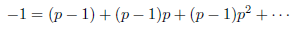
Indeed, set

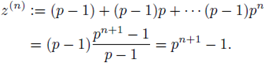
Then lim_n→∞ z⁽ⁿ⁾ = lim_n→∞ pⁿ⁺¹ - 1 = 0 - 1 = -1, since = |pⁿ⁺¹|p = p⁻ⁿ⁻¹.

The unit ball

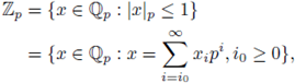
is a ring, more precisely, it is a domain of principal ideals. Any ideal of Zp has the form

Indeed, let be an ideal. Set , and let x₀ ∈ I such that ord(xo) = m₀. Then

From a geometric point of view, the ideals of the form constitute a fundamental system of neighborhoods around the origin in The residue field of is (the finite field with p elements).

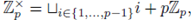
The group ofunits of is

Lemma 2.12. x = x₀ + x₁p + ... ∈ is a unit if, and only if, x ₀ ≠ 0. Moreover if x ∈ \ {0}, then

2.2. Topology of Q _p

As we already mentioned, with d(x,y) = |x → y|_p is a complete metric space. Define

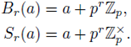
as the ball with center a and radius p^r, and

as the sphere with center a and radius p^r.

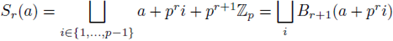
The topology of is quite different from the usual topology of First of all, since the radii are always integer powers of p; for the sake of brevity we just use the power in the notation Br(a) and Sr(a). On the other hand, since the powers of p and zero form a discrete set in in the definition of B_r (a) and S_r (a) we can always use '≤'. Indeed,

Remark 2.13.

We declare B_r(a), r ∈ a ∈ , are open subsets; in addition, these sets form a basis for the topology of .

Proposition 2.14. S_r (a), B_r (a) are open and closed sets in the topology of .

Proof. We first show that S_r(a) is open. Note that then

is an open set.

In order to show that S_r (a) is closed, we take a sequence of points of S_r (a) converging to We must show that Note that Since {x_n} is a Cauchy sequence, we have

thus is also Cauchy, and since Q_P is complete, u_n → Then so in order to conclude our proof we must verify that Because u_m is arbitrarily close to their p-adic expansions must agree up to a big power of p, hence

A similar argument shows that B _r (a) is closed.

Proposition 2.15. f b ∈ B _r (a) then B _r (b) = B _r (a), i.e., any point of the ball B _r (a) is its center.

Proof. Let x ∈ B_r (b); then,

i.e., B_r(b) ⊆ B _r (a). Since a ∈ B_r(b) (i.e. |b - a|_p = |a - b|_p ≤ p^r), we can repeat the previous argument to show that B_r (a) ⊆ B_r (b). 0

Lemma 2.16. The following assertions hold:

(i) any two balls in are either disjoint or one is contained in another;

(ii) the boundary of any ball is the empty set.

Theorem 2.17 ([1, Sec. 1.8]). A set K ⊂ is compact if, and only if, it is closed and bounded in .

2.3. The n-dimensional p-adic space

We extend the p-adic norm to by taking

We define then, ||x||_p = p^-ord(^x). The metric space is a separable complete ultrametric space (here, separable means that contains a countable dense subset, which is ).

For r ∈ denote by the ball of radius p ^r

with center at a = (a₁,...,a_n) ∈ and take Note that where is the one-dimensional ball of radius p^r with center at The ball equals the product of n copies of Bo = . We also denote by the sphere ofradius p^r with center at a = (a₁, . . . , a_n) ∈ , and take We notice that (the group of units of ), but

As a topological space is totally disconnected, i.e., the only connected subsets of are the empty set and the points. Two balls in are either disjoint or one is contained in the other. As in the one dimensional case, a subset of is compact if, and only if, it is closed and bounded in . Since the balls and spheres are both open and closed subsets in Q^J, one has that is a locally compact topological space.

3. Integration on Q _p

For this section we assume a basic knowledge of measure theory (see e.g. ^[26]).

Theorem 3.1 ([26, Thm B. Sec. 58]). Let (G, ·) be a locally compact topological group. There exists a Borel measure dx, unique up to multiplication by a positive constant, such that for every non empty Borel open set U, and for every Borel set E.

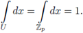
The measure dx is called a Haar measure of G. Since ( , +) is a locally compact topological group, by Theorem 3.1 there exists a measure dx, which is invariant under translations, i.e., d(x + a) = dx. If we normalize this measure by the condition

then dx is unique.

For the n-dimensional case we use that ( , +) is a locally compact topological group. We denote by d ⁿ x the product measure dxi ... dx _n such that

This measure also satisfies that d ⁿ (x + a) = d ⁿ x, for a ∈ The open compact balls of , , generate the Borel σ-algebra of The measure d ⁿ x assigns to each open compact subset U a nonnegative real number which satisfies

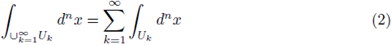
for all compact open subsets U _k in , which are pairwise disjoint, and verify is still compact. In addition,

3.1. Integration of locally constant functions

A function is said to be locally constant if for every x ∈ there exists an open compact subset U, containing x, and such that f (x) = f (u) for all u ∈ U.

Lemma 3.2. Every locally constant function is continuous.

Remark 3.3. Set then I is countable. We fix a set of representatives for the elements of I of the form

If V is an open subset of , then for any x ∈ V there exists a ball contained in V of the form

for some j ∈ I ⁿ and m ∈ containing x. Consequently, is a second-countable space.

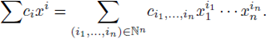
Any locally constant function can be expressed as a linear combination of characteristic functions of the form

where

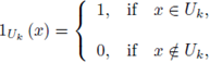
and is an open compact for every k. In the proof of this fact one may use Remark 3.3.

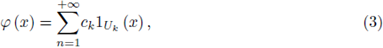
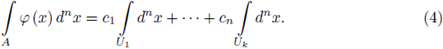
Let be a locally constant function as in (3). Assume that with U_i open compact. Then we define

We recall that, given a function the support of 9 is the set

A locally constant function with compact support is called a p-adic test function or a Bruhat-Schwartz function. These functions form a C-vector space denoted as D. From (2) and (4) one has that the mapping

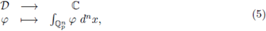
is a well-defined linear functional.

3.2. Integration of continuous functions with compact support

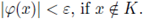
We now extend the integration to a larger class of functions. Let U be a open compact subset of . We denote by C(U, ) the space of all the complex-valued continuous functions supported on U, endowed with the supremum norm. We denote by the space of all the complex-valued continuous functions vanishing at infinity, endowed also with the supremum norm. The function 9 vanishes at infinity, if given ε > 0, there exists a compact subset K such that

It is known that is dense in (see, e.g., [53, Prop. 1.3]). We identify C(U, ) with a subspace of , therefore is dense in C(U, ).

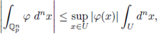
We fix an open compact subset U and consider the functional (5), since

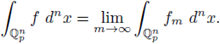
This means that if f ∈ C(U, ) and is any sequence in approaching f in the supremum norm, then

3.3. Improper Integrals

Our next task is the integration of functions that do not have compact support. A is said to be locally integrable, if

exists for every compact K.

Example 3.4. The function |x|_p is locally integrable but not integrable.

Definition 3.5 (Improper Integral). A function is said to be integrable in if

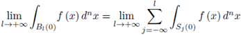
exists. If the limit exists, it is denoted as and we say that the improper integral exists.

Note that

3.4. The change of variables formula in dimension one

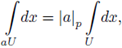
Let us start with the formula

which means the following:

for every Borel set for instance an open compact subset. Consider

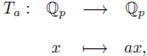
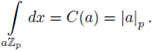
with is a topological and algebraic isomorphism. Then is a Haar measure for ( , +), and by the uniqueness of such measure, there exists a positive constant C(a) such that 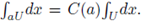To compute C(a) we can pick any open compact set, for instance and then we must show

Let us consider first the case Fix a system of representatives then,

And

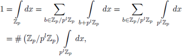
i.e.,

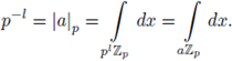
The case is treated in a similar way.

Now, if we take where U is a Borel set, then

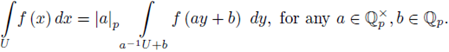
The formula follows by changing variables as x = ay + b. Then we get dx = d (ay + b) = d(ay) = | a|_p dy, because the Haar measure is invariant under translations and formula (6).

Example 3.6. Take U = \ {0}. We show that

Notice that U is not compact, since the sequence converges to 0 ∈ U. Now, by using

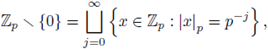
we have

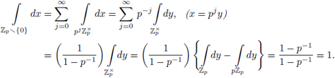
This calculation shows that \ {0} has Haar measure 1 and that {0} has Haar measure 0.

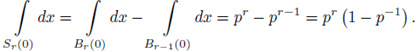
Example 3.7. For any r ∈ ,

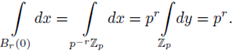
Example 3.8. For any r ∈ ,

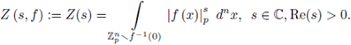
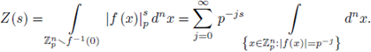
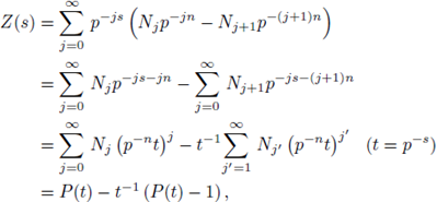
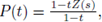
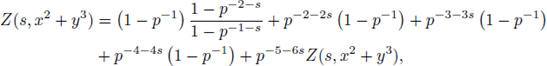
Example 3.9. Set

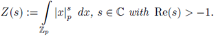
We prove that Z(s) has a meromorphic continuation to the whole complex plane as a rational function of p ^-s .

Indeed,

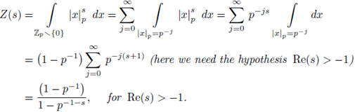
We now note that the right hand-side is defined for any complex number s ≠ -1, therefore, it gives a meromorphic continuation of Z(s) to the half-plane Re(s) < -1. Thus we have shown that Z(s) has a meromorphic continuation to the whole with a simple pole at Re(s) = -1.

Example 3.10. Let be a radial function, i.e., f(x) = f(|x|_p). If then

Example 3.11. By using one may show that

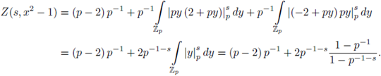
Example 3.12. We compute

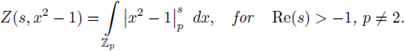
Let us take as a system of representatives of Then,

and

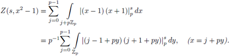
Let us consider first the integrals in which 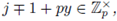i.e., the reduction mod p of j ∓ 1 is a nonzero element of in this case,

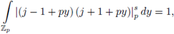
and since p ≠ 2, there are exactly p - 2 of those j's; then,

Lemma 3.13. Take q (x) = FJ (x → a¿)^ei ∈ Z_p [x], a¿ ∈ Z_p, ej ∈ N \ {0}. Assume that Assume that mod p. Then by using the methods presented in examples 3.9 and 3.12, one can compute the integral

3.5. Change of variables (general case)

A function is said to be analytic on an open subset U ⊆ , if there exists a convergent power series with open, such that for In this case, is a convergent power series. A function f is said to be bi-analytic if f and f^-1 are analytic.

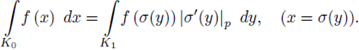
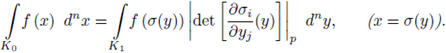
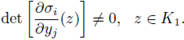
Let K ₀ , K ₁ ⊂ be open compact subsets. Let σ : K ₁ → K ₀ be a bi-analytic function such that σ '(y) ≠ 0, y ∈ K ₁ . Then, if f is a continuous function over K₀,

4. Implicit Function Theorems on Q _p

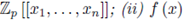
Let us denote by [[x₁,..., x_n]], the ring of formal power series with coefficients in . An element of this ring has the form

A formal series is said to be convergent if there exists r ∈ Z such that converges for satisfying ||a||_p = max_i |a _i | _p < p ^r . The convergent series form a subring of [[x₁,...,x_n]], which will be denoted as

If for there exists such that for all we say that is a dominant series for and write

Proposition 4.1. A formal power series is convergent if, and only if, it has a dominant series.

Proof. Set Assume that then

and thus is convergent by Lemma 2.10.

If then there exists r ∈ such that converges for any ||a|| _p < p^r. Choose r₀ ∈ such that 0 < p^r0 < p^r. Then for every a ∈ satisfying ||a|| _p < p^r0 , we have

and thus Hence, for some positive constant M. Finally,

We say that is a special restricted power series, abbreviated SRP, if f (0) = 0, i.e., c₀ = 0, and c_i = 0 mod p ^|i|−1 , for any

Lemma 4.2. Assume that f (x) is a SRP; then the following assertions hold: (i) f (x) ∈ is convergent at every a in

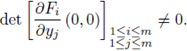
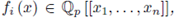
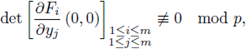
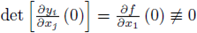
Theorem 4.3 (First Version of the Implicit Function Theorem). (i) Take F (x,y) = (Fi (x,y),..., F_m (x, y)), with such that F _i (0, 0) = 0, and

Then there exists a unique f (x) = (f _i (x),..., f _m (x)), with f _i (0) = 0, satisfying F (x, f (x)) = 0, i.e., F _i (x, f (x)) = 0 for all i.

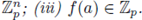
(ii) If each Fi (x, y) is a convergent power series, then every fi (x) is a convergent power series. Furthermore, if a is near 0 in then f (a) is near 0 in and F (a, f (a)) = 0; and if (a, b) is near (0, 0) in and F (a, b) = 0, then b = f (a).

For a proof of this result the reader may consult [31, Thm. 2.1.1].

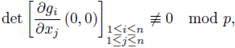
Corollary 4.4 ([31, Cor. 2.1.1]). for 1 ≤ i ≤ n, and

then there exists a unique f (x) = (f _i (x),...,f _n (x)) with f _i (x) ∈ [[x _i ,...,x _n ]], fi (0) = 0, for all i, such that g (f(x)) = x.

(ii) If then for all i. Furthermore, if b is near 0 in and a = g(b), then a is also near 0 in and b = f(a). Therefore, y = f (x) gives rise to a bi-continuous map from a small neighborhood of 0 in to another neighborhood of 0 in .

Remark 4.5. (i) Take open subsets containing the origin. Assume that each F _i (x,y) : U ₁ x U ₂ → is a convergent power series. A set of the form

is called an analytic set. In the case in which all the Fi (x, y) are polynomials and is called an algebraic set. If all the satisfy the hypotheses of the implicit function theorem, V has a parametrization, possible after shrinking U₁, U₂, i.e. there exist open subsets containing the origin 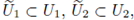such that

(ii) If we now use as coordinates

we have

We say that such V is a closed analytic submanifold of of codimension m. The word 'closed' means that V is closed in the p-adic topology.

In the next version of the implicit function theorem we can control the radii of the balls involved in the theorem.

Theorem 4.6 (Second Version of the Implicit Function Theorem). (i) If F _i (x,y) ∈ for all i and

then there exists a unique solution f (x) = (f ₁ (x),..., f _m (x)), with f _i (x) ∈ of F (x,f (x)) = 0, i.e. Fi (x, f (x)) = 0 for all i.

(ii) If every F _i (x, y) is an SRP in x ₁ ,..., x _n ,y ₁ ,...,y _m , then every f _i (x) is an SRP in x ₁ ,...,x _n . Furthermore, if a ∈ then f (a) ∈ and F (a, f (a)) = 0, and if (a, b) ∈ satisfies F(a, b) = 0, then b = f (a).

For a proof of this result the reader may consult [31, Thm. 2.2.1].

Corollary 4.7 ([31, Cor. 2.2.1]). (i) If for all i, and further

then every f _j (x) in the unique solution of g _i (f ₁ (x),..., f _n (x)) = x satisfying f _j (0) = 0 is also in

(ii) If every gi(x) is a SRP in x1, . . . , xn, then every fj(x) is also a SRP in the same variables, and, y = f(x) gives rise to a bi-continuous map from to itself.

Remark 4.8. Assume that every F _i (x,y) is a SRP in x,y. Take

Under the hypotheses of the second version of the implicit function theorem, we have

By using the coordinate system

V takes the form

and we will say V is a closed analytic submanifold of of codimension m.

4.1. General change of variables formula

Theorem 4.9 ([31, Prop. 7.4.1]). Let K ₀ , K ₁ ⊂ be open compact subsets, and let σ = (σ1, . . . , σ_n) : Ki → K₀ be a bi-analytic map such that

If f is a continuous function on K ₀ , then

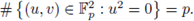
5. The Igusa local zeta functions

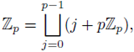
Let p be a fixed prime number. Set

the ring of integers modulo p ^m . Recall that any integer can be written in a unique form as

Thus we can identify, as sets, A_m with

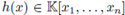
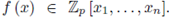
Take f (x) ∈ [x₁,..., x_n] \ , and define

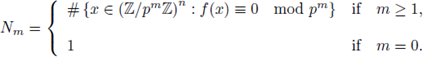
A basic problem is to study the behavior of the sequence N _m as m → ∞.

More generally, we can take f (x) ∈ _p [x₁,... ,x_n] \ _p (recall that ⊂ _p and that 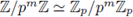), and

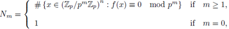
where x = y mod p^m means x → y ∈ p^m _p. To study the sequence we introduce the following Poincaré series:

We expect that the analytic properties of P(t) provide information about the asymptotic behavior of the sequence . A key question is the following:

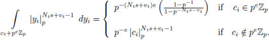
In what follows we will use the convention: given a > 0 and s ∈ we set

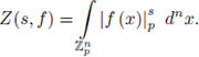
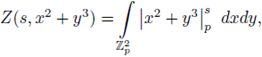
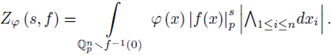
Definition 5.1. Let and let 92 be a locally constant function with compact support, i.e., an element of The local zeta function (also called Igusa's local zeta function) attached to (f, φ) is

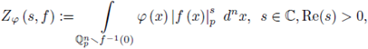
where dⁿx is the Haar measure of ( , +) normalized such that

Remark 5.2. Z _φ (s, f) is an holomorphic function on the half-plane Re(s) > 0. For the proof of this fact the reader may consult [31, Lemma 5.3.1].

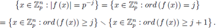
Given we set

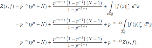
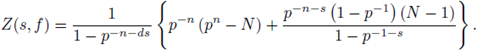
Proposition 5.3. With the above notation,

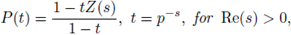
where P(t) is the Poincaré series defined in (7).

Proof. We first note that

On the other hand,

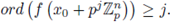
Now, take satisfying ord (f (x₀)) ≥ j, then, by using Taylor expansion,

we have ord (f (x₀ + p^jz)) ≥ j, for all z ∈ i.e. This fact implies:

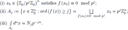
Therefore,

i.e., for Re(s) > 0. 0

Theorem 5.4 (Igusa, [31, Thm. 8.2.1]). Let f (x) be a non-constant polynomial in There exist a finite number of pairs such that

is a polynomial in p ^-s with rational coefficients.

The proof of this theorem will be given in Section 8. From Theorem 5.4 and Proposition 5.3, we get:

Corollary 5.5. P(t) is a rational function of t.

The rationality of P(t) was conjectured in the sixties by Borevich and Shafarevich. Igusa proved this result at middle of the seventies. The rationality of Z _φ (s, f) also allows us to find bounds for the N_m's (see e.g. ^[28] and ^[31]).

The proof of Theorem 5.4 given by Igusa depends on a deep result in algebraic geometry known as Hironaka's resolution of singularities theorem. Now we introduce the stationary phase formula, which is an elementary method for computing p-adic integrals like Z _φ (s, f), Igusa has conjectured in ^[29] that this method will conduct to a new elementary proof of the rationality of Z _φ (s, f).

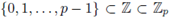
6. The Stationary Phase Formula

Let us identify F_p, set-theoretically, with {0,1,... ,p - 1}. Let '-' denote the reduction mod p map, i.e.,

This map can be extended to The reduction mod p of a subset will be denoted as denotes its reduction mod p.

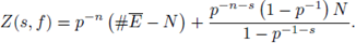
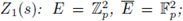
Proposition 6.1 (Stationary Phase Formula). Take and denote by the subset consisting of all such that 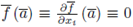mod p, for 1 ≤ i ≤ n. Denote by E, S the preimages of under reduction mod p map and by N the number of zeros of Then

Proof. By definition then,

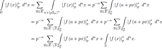
Take such that in this case,

and the contribution of these

Take now

say i = 1. Define

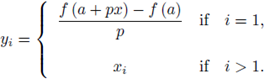
Then y_i's are SRP's and mod p; hence, the map x → y gives rise to a measure-preserving map from to itself (cf. Corollary 4.7). Therefore,

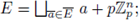
and the contribution of the points of the form (8) is

Set The stationary phase formula, abbreviated SPF, can be re-written as

We can now apply SPF to each Igusa has conjectured that by applying recursively SPF, it is possible to establish the rationality of integrals of type in the case in which the polynomial f has coefficients in a non-Archimedean complete field of arbitrary characteristic.

The arithmetic of the Laurent formal series field

is completely analog to that of . In particular, given a polynomial with coefficients in we can attach to it a local zeta function, which is defined like in the p-adic case. The rationality of such local zeta functions is an open problem. The main difficulty here is the lack of a theorem of resolution of singularities in positive characteristic. The above-mentioned conjecture can be re-stated saying that the rationality of local zeta functions for polynomials with coefficients in should follow by applying recursively SPF.

Remark 6.2. Take If the system of equations

has no solutions in then S = ∅, and by SPF,

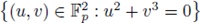
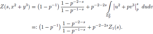
Example 6.3. Let be a homogeneous polynomial of degree d, such that implies We now compute Z(s, f). We use SPF with

therefore,

6.1. Singular points of hypersurfaces

Take

and define

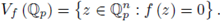
Vf ( ) is the set of -rational points of the hypersurface defined by f. This notion can be formulated on an arbitrary field K. Set

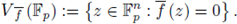
is the set of F_p-rational points of the hypersurface defined by If

then A point a ∈ Vf ( ) is said to be singular if for 1 ≤ i ≤ n. The set of singular points of Vf ( ) is denoted as Sing _f ( ). We define In a similar form we define

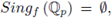
Note that . In fact, it may occur that and that For instance, if f (x,y) = px + x ² → y ³ , then , but

Example 6.4. We compute Z(s, f) for f (x, y) = px + x² - y ³ by using SPF. Note that

then, by applying SPF,

By changing variables in the last integral as x = pu, y = pv, we have

We now apply SPF to the last integral. Take Since the system ofequations

has no solutions, by applying SPF we get

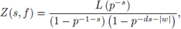
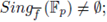Remark 6.5. Take If but then,

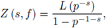
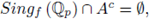
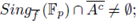
where L (p ^-s ) is a polynomial in p^-s with rational coefficients (see ^{[60]- [61]}). The denominator of Z (s, f) is controlled by Nowadays the numerator is not fully understood, but it depends strongly on The lack of -singular point, i.e. Sing _f ( ) = ∅, makes the denominator of Z (s,f) 'trivial': 1 or 1 → p^-1-s.

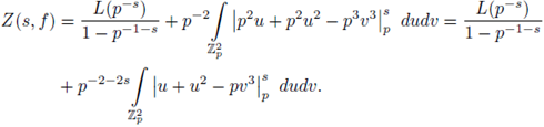
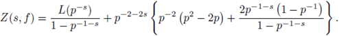
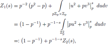
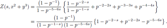
Example 6.6. We now compute

by using SPF. Note that and that

because the set can be parametrized as u = α ³ , v = α ² , with By applying SPF we have

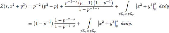
By changing variables in the last integral as x = pu, y = pv, dxdy = p ^-2 dudv,

We now apply SPF to since the solution set of u ² = 2u = 0 is then In addition, Therefore,

and

We now apply SPF to then,

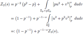
and

Finally, we apply SPF to then,

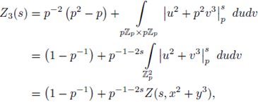
and

i.e.,

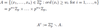
6.2. Quasi-homogenous singularities

Take and We say that f(x) is a quasi-homogeneous polynomial of degree d with respect to w if: (1) .

Set |w| := w₁ + ... + w_n, and

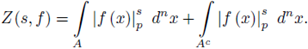
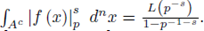
Proposition 6.7. With the above notation and hypotheses,

where L (p^-s) is a polynomial in p ^-s with rational coefficients.

Proof. Set

Then,

By changing variables in the first integral as we have

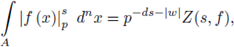
And

We now note that but it may occur that this makes the computation of the integral on A^c not simple. By using SPF recursively and some ideas on Néron p-desingularization, one can show that For a detailed proof, including the most general case of the semiquasi-homogeneous singularities, the reader may consult ^[60].

7. p-adic Analytic Manifolds and Resolution of Singularities

This section is based on [31, Sec. 2.4]. Let be a non-empty open set, and let f : U → be a function. If at every point a = (a₁,...,a_n) of U there exists an element such that f (x) = f_a(x) for any point x near to a, we say that f is an analytic function on U. It is not hard to show that all the partial derivatives of f are analytic on U.

Let U be as above and let h = (h₁,..., h_m) : U → be a mapping. If each h _i is an analytic function on U, we say that h is an analytic mapping on U.

Let X denote a Hausdorff space and n a fixed non-negative integer. A pair (U, ф _U ), where U is a nonempty open subset of X and ф _U : U → ф _u (U) is a bi-continuous map (i.e., a homeomorphism) from U to an open set is called a chart. Furthermore ф _U (x) = (x₁,..., x_n), for a variable point x of U are called the local coordinates of x. A set of charts {(U, ф _U )} is called an atlas if the union of all U is X and for every U, U' such that U ∩ U' ≠ ∅ the map

is analytic. Two atlases are considered equivalent if their union is also an atlas. This is an equivalence relation and any equivalence class is called an n-dimensional p-adic analytic structure on X. If {(U, ф _U )} is an atlas in the equivalence class, we say that X is an n-dimensional p-adic analytic manifold, and we write n = dim (X).

Suppose that X, Y are p-adic analytic manifolds respectively, defined by {(U, ф _U )}, {(V, ψv)}, and f : X → Y is a map. If for every U, V such that U ∩ f^-1 (V) ≠ ∅ the map

is analytic, then we say that f is an analytic map. This notion does not depend on the choice of atlases.

Suppose that X is a p-adic analytic manifold defined by {(U, ф _U )} and Y is a nonempty open subset of X. If for every U' = Y ∩ U ≠ ∅ we put ф _U' = ф _U | _U’ , then {(U', ф _U’ ')} gives an atlas on Y, which makes Y a p-adic analytic open submanifold of X, with dim(X) = dim(Y).

If U, U^' are neighborhoods of an arbitrary point a of X, and f, g are p-adic analytic functions respectively on U, U' such that f |_W = g |_W for some neighborhood W of a contained in U ∩ U^', then we say that f, g are equivalent at a. An equivalence class is

said to be a germ ofanalytic functions at a. The set of germs of analytic functions at a form a local ring denoted by or simply

Suppose that Y is a nonempty closed subset of X, a p-adic analytic manifold as before, and 0 < m ≤ n such that an atlas {(U, ф _U )} defining X can be chosen with the following property: If ф _U (x) = (x₁,...,x_n) and U' = Y ∩ U ≠ ∅, there exist p-adic analytic functions F₁,..., F_m on U such that firstly U' becomes the set of all x in U satisfying F₁ (x) = ... = F_m (x) = 0, and secondly,

Then by Corollary 4.4-(ii) the mapping x → (F₁ (x),..., F_m (x), x_m+1,..., x_n) is a bi-analytic mapping from a neighborhood of a in U to its image in If we denote by V the intersection of such neighborhood of a an Y, and put Ψ_V (x) = (x_m+1,... , x_n) for every x in V, then {(V, Ψ_V)} gives an atlas on Y. Therefore Y becomes a p-adic analytic manifold with dim (Y) = n - m. We call Y a closed submanifold of X of codimension m.

Let µ_n denote the normalized Haar measure of Take X and {(U, ф _U )} as before. Set a a differential form of degree n on X; then α |_U has an expression of the form

in which f_U is an analytic function on U. If A is an open and compact subset of X contained in U, then we define its measure µ α (A) as

We note that the above series converges because f_u (A) is a compact subset. If (U', ф _U’ ) is another chart and A ⊂ U’ then we will have the same µ_α (A) relative to that chart. In fact, if then

Actually, the previous equations just give account of the change of variables rule as x → x', in the integral (9), that is

(see [31, pg. 112 and Proposition 7.4.1]). Note that if and

then µ_α is the normalized Haar measure of

Theorem 7.1 (Hironaka). Take f (X) a nonconstant polynomial in [x₁,...,x_n], and put X = Then there exist an n-dimensional p-adic analytic manifold Y, a finite set T = {E} of closed submanifolds of Y of codimension 1 with a pair of positive integers (N _E ,V _E ) assigned to each E, and a p-adic analytic proper mapping h : Y → X satisfying the following conditions: (i) h is the composition of a finite number of monoidal transformations each one with a smooth center; (ii)

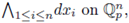
and h induces a p-adic bianalytic map

(iii) at every point b of Y, if E₁,...,E_m are all the E in T containing b with local equations y ₁ ,...,y _m around b and (N _i , v _i ) = (N_E , v _E ) for E = Ei, then there exist local coordinates of Y around b of the form (y ₁ ,...,y _m ,y _m+1 ,…,y _n ) such that

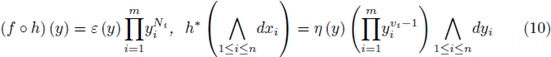
on some neighborhood of b, in which ε (y), r, (y) are units of the local ring of Y at b. In particular, has normal crossings.

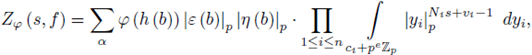
8. Proof of Theorem 5.4

We want to end this notes by proving Igusa's Theorem about the meromorphic continuation of Z _φ (s, f) (see Theorem 5.4 in Section 5). We follow the proof given by Igusa in [31, Thm. 8.2.1].

Let denote the measure induced by the differential form which agrees with the Haar measure of Then

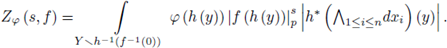
Pick a resolution of singularities h : Y → Xi for f ^-1 (0) as in Theorem 7.1; we use all the notation introduced there. Then Y \ h ^-1 (f ^-1 (0)) → X \ f ^-1 (0) is a p-adic bianalytic proper map, i.e., a proper analytic coordinate change; then,

At every point b of Y \ h ^-1 (f ^-1 (0)) we can choose a chart (U, (ф _U ) such that (10) holds. Since h is proper and the support of φ, say A, is compact, we see that h ^-1 (A) := B is compact. Then we can cover B by a finite disjoint union of open compact balls B _a such that each of these balls is contained in some U above. 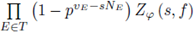Since φ is locally constant, after subdividing B _α we may assume that and further that for some c = (c ₁ ,..., c _n ) in and Then,

with the understanding that N _i = 0,v _i = 1 in the case E _i is not crossing through b. Finally one has by [31, Lemma 8.2.1] that