English (pdf)
 Article in xml format
 Article references
 Send this article by e-mail
 Cited by SciELO
  Cited by Google
  Similars in
SciELO
Similars in
SciELO  Similars in Google
 Permalink
INTRODUCTION
Phenology is the study of recurrent biological events in the life cycle of plants and animals, and their relationship with biotic and abiotic factors (Denny et al., 2014). Flowering is one of these events, and flowering phenology has been widely studied in different life forms, such as trees, shrubs and herbs. They all show similar variation patterns regarding the onset, duration and end of the flowering period in response to changes in temperature and humidity along elevation gradients (Cornelius et al., 2013; Cortés-Flores et al., 2017). Thanks to the existing studies on the subject, it is now possible to understand the influence of biotic factors like pollinators and herbivores (Elzinga et al., 2007; Cortés-Flores et al., 2017), and abiotic factors like water and light availability (Galloway and Burgess, 2012; Valentin-Silva et al., 2018) on the flowering phenology of plants.
There is a significant body of evidence showing that flowering phenology is affected by temperature and the availability of water and light (Ramírez, 2002; Cascante-Marín et al., 2017; Cortés-Flores et al., 2017; Zhou et al., 2019). In elevational gradients where water availability and temperature vary, it is possible to observe intraspecific variation in different phenological traits (Taffo et al., 2019; Rafferty et al., 2020). For example, due to the lower temperatures which occur at high elevations, populations of trees, shrubs and herbs display delayed flowering start dates compared to populations at lower elevations (Cornelius et al., 2013; Bucher et al., 2017; Singh and Mittal, 2019).
For vascular epiphytes-plants that lives on other plants without taking nutrients directly from them (Zotz, 2016)- flowering phenology has barely been studied (Sheldon and Nadkarni, 2015; Cascante-Marín et al., 2017), and patterns related to elevational gradients are unknown. Vascular epiphytes differ from other plant life forms in their reliance on alternative sources of water and nutrients (e.g., fog, dew, throughfall and stemflow) (Van Stan II and Pypker, 2015; Wu et al., 2018), and their susceptibility to the microenvironment provided by the tree host (phorophyte) (Wagner et al., 2015; Ticktin et al., 2016; Rasmussen and Rasmussen, 2018). Given these differences, it could be expected for vascular epiphytes to also display distinct elevational patterns in their phenology.
Vascular epiphytes represent 9 % of the world's diversity of vascular plants (Zotz, 2016), and they are key components for ecosystem functions because they affect the nutrient and water cycles (Van Stan II and Pypker, 2015; Petean et al., 2018). Furthermore, vascular epiphytes enhance biodiversity by providing food, shelter and water to numerous organisms ranging from bacteria to vertebrates (Cruz-Ruiz et al., 2012; Corbara et al., 2019).
To broaden our understanding of vascular epiphyte phenology, we described the phenological patterns of Tillandsia carlos-hankii Matuda, a tank epiphytic bromeliad, along an elevation gradient in Capulálpam de Méndez in Oaxaca, Mexico. Our analyses were directed to respond the following questions: 1) How do flowering start date, duration and seasonality vary along the gradient? 2) Given that vascular epiphytes are very sensitive to microclimatic variation (Wagner et al., 2015; Zotz, 2016; Ramírez-Martínez et al., 2018), which phenologycal variables are more prone to show intra-population differences within the same elevation range? 3) Considering reports showing that phorophyte size can influence the richness and abundance of epiphytes (Flores-Palacios and García-Franco, 2006; Ortega-Solís et al., 2020), how the start date and duration of flowering are affected by the height, diameter at breast height (DBH) and canopy diameter of phorophyte?
MATERIALS AND METHODS
Study site
Capulálpam de Méndez is located in the Sierra Norte region of Oaxaca (17°18' N, 96° 27' W) in Mexico, within an elevation range of 1100-3200 meters above sea level (m. a. s. l.). Local climate is sub-humid temperate, with rain in the summer C , Median annual precipitation is 1 115 mm, and average annual temperature is 15.2 °C (Santiago, 2009). Seasonality consists of a rainy season from May to October and a dry season from November to April (López-López, 2017).
On the western part of the territory of Capulálpam de Méndez, we established six sampling plots along three elevation ranges (hereafter referred to as zones): low, medium and high (two plots on each elevation). The area is covered by a pine-oak forest, with representative species of the genera Pinus, Quercus and Arbutus. The epiphytic bromeliad community is comprised by T. carlos-hankii, T. prodigiosa (Lem.) Baker, T. calothyrsus Mez., T. macdougallii L.B.Sm., T. gymnobotrya Baker, T. oaxacana L.B.Sm., T. violacea Baker, T. bourgaei Baker, Viridantha plumosa (Baker) Espejo and Catopsis sp. (López-López, 2017) (Table 1). Tillandsia carlos-hankii was chosen as the study species because it has a narrow distribution range, there are abundant populations in the study area, it is endemic to the state of Oaxaca, it is classified as threatened species in the Mexican legislation (NOM-059-SEMARNAT-2010) and it is used locally.
Table 1 Description of the vegetation in the sampling plots (100 m2) established at each site in Capulálpam de Méndez (López-López, 2017).
*Standard Deviation
Study species
Tillandsia carlos-hankii is a stemless, monocarpic, tank epiphytic bromeliad endemic to Oaxaca. It grows in pine-oak forests between 1900 to 2900 m. a. s. l. (Espejo-Serna et al., 2004). The leaves form a dense rosette, 40-89 cm high; the stalk is sturdy, 57-70 cm long, with imbricate green broad bracteae at the base which gradually become red and narrow towards the tip. It produces trochilophilous tubular flowers with exerted stamens and style. Fruits are capsules with wind dispersed seeds (Fernández-Ríos, 2012). At the study site, the species grows on Quercus and Pinus phorophytes (Ramírez-Martínez et al., 2018).
Field work
First, we identified the distribution limits of T. carlos-hankii along the elevation gradient in Capulálpam de Méndez. Once we knew the local distribution range for the species, we defined three elevation zones: "low" 2151 to 2283 m. a. s. l., "medium" 2284 to 2416 m. a. s. l. and "high" 2417 to 2548 m. a. s. l. (Table 1). Each elevation zone represented approximately 100 m. a. s. l., to ensure we captured variation in environmental conditions based on a study which reported a decrease of 0.7 °C for each 100 m elevation-increase in a location near the study site (Zacarías-Eslava and Del Castillo, 2010). For each elevation zone, we selected two populations of T. carlos-hankii with the same sun orientation (Table 1). We considered each patch of T. carlos-hankii as a separate population because this species lives in discontinuous patches in the area, and studies indicate that seed dispersal in epiphytic bromeliads is limited (Mondragón and Calvo-Irabien, 2006). Distances between populations ranged from 0.4 to 2.84 km. A vegetation analysis conducted in the study site (López-López, 2017), revealed that dominant tree species varied within and between elevations (e.g. there was a higher percentage of oak trees at the lower elevations).
Phenology monitoring
Quercus trees are preferred phorophytes for T. carlos-hankii (Ramírez-Martínez et al., 2018). Because Quercus trees are abundant in the study site but there are few trees per species, we only sampled individuals of T. carlos-hankii growing on Quercus spp., to minimize the potential effect of the phorophyte on flowering phenology. As there is no standard methodology to monitor the flowering phenology of vascular epiphytes, we randomly selected 63 ± 16 (mean ± SD) adult individuals of T. carlos-hankii in the vegetative state, in each of the six populations studied (between 51 to 88 individuals per population). Based on a previous study (Ramírez-Martínez et al., 2018), all individuals measuring at least 50 cm from the base ofthe plant to the tip of the longest immature leaf (because mature leaves were curved) were considered adults. We then monitored their phenological status periodically.
To minimize potential differences in phenological responses related to microenvironmental conditions and height within the phorophyte, we only sampled individuals of T. carlos-hankii attached at heights between 0.30 to 3.80 m (mean=2.02 m ±0.93 m). This height range corresponds to Johansson zone II, where microenviromental conditions are expected to be similar (Zotz, 2016). Each phorophyte was labeled with a specific ID code. On each phorophyte we selected one to three adult individuals. Every selected individual was labeled with an ID tag indicating a unique code conformed by the ID of the phorophyte on which it was growing and an individual code to distinguish between different bromeliads found on the same tree.
To test if phorophyte traits influenced the flowering phenology of T. carlos-hankii (start and duration), for each tagged tree we recorded phorophyte height, DBH (Diameter at Breast Height at 1.30 m) and canopy diameter.
From June 2016 to May 2017, we monitored all the selected individuals monthly, excepting in November when monitoring was done weekly because we knew, from previous experience, that T. carlos-hankii could begin producing flowers. Whenever we observed an individual with flower buds, we shifted to a daily census schedule for that individual, to ensure accurate records of flowering start date and duration. Flowering start date was defined by the emergence of floral buds, flowering end date was recorded when all the flowers were senescent, and flowering duration was measured as the number of days between the appearance of the first floral bud and the last open flower. For this purpose, during monitoring we recorded the daily number of flower buds, open flowers and senescent flowers for each individual.
Data analysis
Variation in flowering start date and effects of phorophyte traits
Circular statistics are recommended to analyze cyclic phenomena. In this study, we applied circular statistics to describe the flowering phenology pattern across and within elevation zones. We converted each day to an angle, so that our circumference was divided into 365 equal intervals of 0.98° (Zar, 2010).
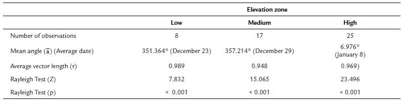
To establish if there were differences in flowering start date across elevation zones (for this analysis, data from the two populations at each elevation zone were pooled together), and between populations at the same elevation, we first calculated the average flowering start date as the mean angle (ᾱ). Then we applied the Rayleigh test (Z), to establish if the distribution of flowering start dates was uniformly dispersed throughout the year, or clustered around a specific period (this test is the most recommended for unimodal data). Additionally, we calculated the longitude of the mean vector (r), which tells us how clustered the flowering start date ofthe individuals from each elevation zone and each population was. Values for this longitude vector range from zero to one: values near one indicate that flowering start dates for most individuals were clustered near the mean flowering start date of the sample (Morellato et al., 2010; Zar, 2010).
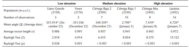
The Mardia-Watson-Wheeler (W) test was used to enquire if the distribution of flowering start dates differed statistically between and within elevation zones. This test compares the mean angle (ᾱ) of different samples (Zar, 2010). Although we tagged more than 50 individual of T. carlos-hankii per population, few tagged individuals produced inflorescences during the sampling period (in total we tagged 381 individuals, but only 50 produced flowers, i.e. only 13 %). Because at least ten individuals are necessary per sample for this analysis, it was not possible to apply the test to compare between low (sample size = 8 individuals) and medium elevations (sample size = 17 individuals), and between low and high elevations (sample size = 25 individuals), only between medium and high elevations. This problem also prevented the comparison between populations within each elevation zone (Llano Grande = 3 individuals vs Yuvee = 5 individuals, Ciénega Baja 2 = 7 individuals vs Ciénega Baja 1 = 10 individuals, and Ciénega Alta = 9 individuals vs Latzieta = 16 individuals). All circular statistics analyses were carried out with the software Oriana version 4.02 (Kovach, 2011).
To evaluate if there were statistical differences in flowering start date between elevation zones and populations (nested on elevations), we applied a General Linear Model (GLM) with a log normal error type. To test for the effect of phorophyte traits on average flowering start date, we included phorophyte height, DBH and canopy diameter as covariables in the model. We ran our analysis in the program SAS version 9.1 (SAS, 2002).
Seasonal variation, flowering duration, and the effect of phorophyte traits on flowering duration
To establish if flowering was seasonal (occurring during a specific period of the year) or uniformly distributed all year around (Morellato et al., 2010), we analyzed the daily frequency of flowering individuals per elevation zone, and for each population within elevation zones. We calculated average flowering date using the mean angle (ᾱ), which shows the day of the year when most individuals were flowering. To test for seasonality, we used the Rayleigh test (Z) and the intensity of seasonality was calculated with the longitude of the mean vector (r). Lastly, to determine if there were statistical differences in seasonality between elevation zones (low vs medium, low vs high, and medium vs high), and between populations in the same elevation zone (i.e. Llano Grande vs Yuvee, Ciénega Baja 2 vs Ciénega Baja 1, and Ciénaga Alta vs Latzieta), we used the Mardia-Watson-Wheeler test (W) (Morellato et al., 2010; Zar, 2010).
We also tested for differences in flowering duration between elevations and between populations (nested by elevation) using a Generalized Linear Model (GLM) with a Log normal error. For pairwise comparisons we used a paired t test, with the function p/diff on the SAS 9.1 software (SAS, 2002). To test for the effect of phorophyte features on flowering duration, we included phorophyte height, DBH and canopy diameter as co-variables in the model.
RESULTS
Variation in flowering start date and effects of phorophyte traits
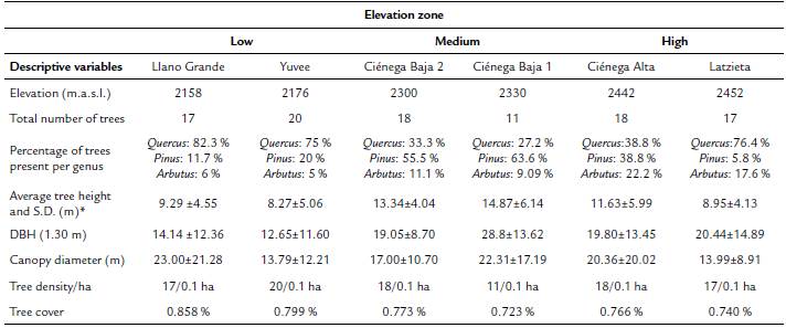
Regarding elevation differences in the onset of flowering, we found that average flowering start date was December 23 for the low elevation zone, December 29 for the middle zone, and January 8 for the high elevation zone (mean angle value (ᾱ), Fig. 1, see Appendix 1). The mean angle date difference between low and medium elevation individuals was six days, between low and high elevation individuals it was 16 days, and between medium and high elevation individuals it was ten days. Most individuals in each elevation zone, started to flower at the same time (r value, Fig. 1, see Appendix 1). Even though the observed pattern suggests that low elevation individuals started flowering earlier than individuals at higher elevations, differences in mean angle values for the medium and high elevation zones were not statistically significant (W = 3.144, p = 0.18). This result was supported by the GLM which also showed no significant differences in flowering start date between elevation zones (F2,44 = 1.71, p = 0..19).
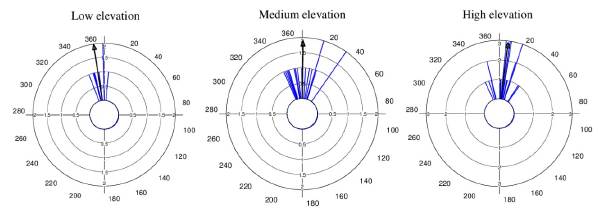
Figure 1 Circular histograms of the flowering start date for T. carlos-hankii for each elevation zone. The length of the blue lines represents the frequency of individuals at their flowering start date; the black arrow indicates the direction (ᾱ ) and the length of the vector (r). The numbers around the circumference indicate the 365 days of the year (each day represents 0.98 ° of the circumference).
Average flowering start dates were very similar between the two populations at low elevation (December 22 and December 23), and between the two populations at high elevation (January 7 and January 8). However, the two populations at medium elevation showed a difference of 13 days in their average flowering start dates (December 21 and January 3) (mean angle value ᾱ, Fig. 2, see Appendix 2). R values showed a high concentration of the flowering start date for most individuals in each population (Fig. 2, see Appendix 2). GLM results did not show statistically significant differences in flowering start dates between populations (F3,44 = 1.96, p = 0.13).
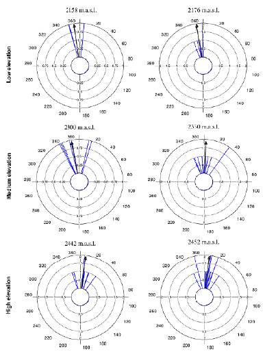
Figure 2 Circular histograms of the flowering start dates of T. carlos-hankii in each population per elevation zone. The length of the blue lines represents the frequency of individuals at their flowering start date, the black arrow indicates the direction (ᾱ ) and the length of the vector (r). The numbers around the circumference indicate the 365 days of the year (each day represents 0.98 ° of the circumference).
None of the phorophyte features analyzed had a significant effect on flowering start date (t ≤ -1.47, p ≥ 0.14, in all cases).
Seasonal variation, flowering duration, and the effect of phorophyte traits on flowering duration
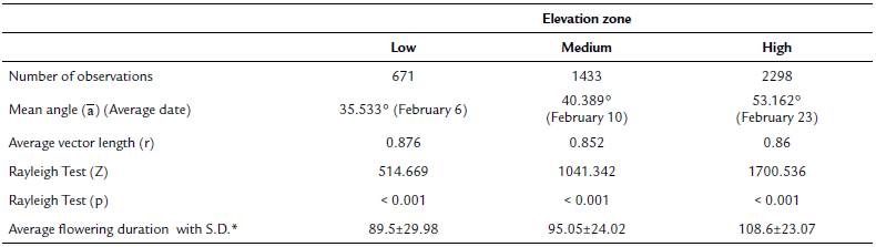
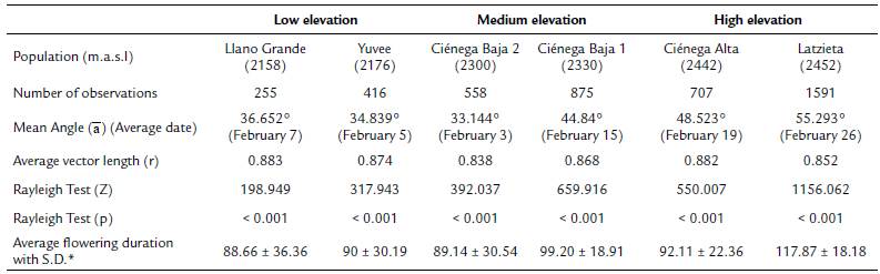
Tillandsia carlos-hankii flowered between December and May. We found evidence of strong seasonality in the three elevation zones (Fig. 3), with a high concentration of individuals flowering simultaneously (r values, Fig. 3, see Appendix 3). Flowering was recorded from December 10 to April 26 in the low elevation zone, from December 3 to May 9 at medium elevation and from December 7 to May 31 at high elevation. The Rayleigh test showed that the seasonality effect was statistically significant for all elevation zones (p < 0.001, see Appendix 3), therefore flowering was seasonal at all elevations. At the same time, the Mardia-Watson-Wheeler test indicated significant differences in seasonality between elevation zones (low vs medium elevation W = 18.498, p < 0.0001; low vs high elevation W = 61.159, p < 0.0001, medium vs high elevation W = 29.963, p < 0.0001. Similarly, all the populations showed a seasonality effect (Fig. 4, see Appendix 4), but seasonality was only simultaneous in the two populations at low elevation. Conversely, tests indicated inter-population variation in the occurrence of the flowering season at medium (W = 33.918, p <0.05), and high (W = 8.579, p = 0.014) elevations.
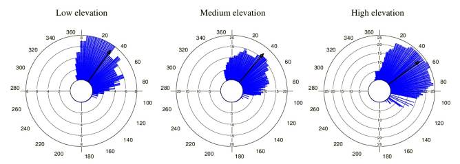
Figure 3 Circular histograms of the flowering of T. carlos-hankii in each elevation zone. The length of the blue lines represents the frequency of individuals in bloom per day, the black arrow indicates the direction (☒) and the length of the vector (r). The numbers around the circumference indicate the days of the year (each day represents 0.98 ° of the circumference).
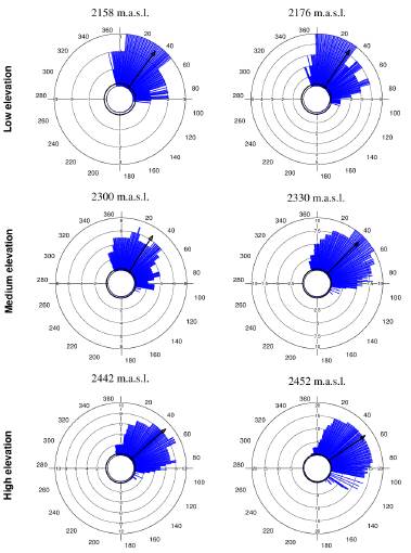
Figure 4 Circular histograms of the flowering of T. carlos-hankii for each population and elevation zone. The length of the blue lines represents the frequency of individuals in bloom per day, the black arrow indicates the direction (ᾱ) and the length of the vector (r). The numbers around the circumference indicate the 365 days of the year (each day represents 0.98 ° of the circumference).
Flowering duration spanned five months in low and medium elevations, and six months in high elevations. Average duration of flowering was significantly different between elevations (F2,44 = 5.26, p < 0.01), but pairwise comparison indicated it was similar in low and medium elevations (t = 0.8, p = 0.42), but different in low and high elevations (t = -2.76, p 0.01), and between medium and high elevations (t =2.5, p = 0.01) (see Appendix 3). Differences in average flowering duration between populations in the same elevation zone were not statistically significant (F3,44 = 0.99, p = 0.40) (see Appendix 4).
None of the analyzed phorophyte features showed a significant effect on flowering duration (t ≤ -1.47, p ≥ 0.14, in all cases).
DISCUSSION
Variation in flowering start date and effect of phorophyte traits
The elevational pattern observed for T. carlos-hankii was similar to patterns reported for other life forms (Ranjitkar et al., 2012; Cornelius et al., 2013; Bucher et al., 2017; Singh and Mittal, 2019). At lower elevations, individuals start flowering earlier than individuals at higher elevations. The presence of this phenological response pattern, which has been related to changes in temperature along the elevational gradient (Cornelius et al., 2013; Bucher et al., 2017), could also be influenced by changes in other factors along the gradient (Ranjitkar et al., 2012; Cascante-Marín et al., 2017; Basnett et al., 2019). We acknowledge that our results could be affected by the relatively small sample size, due the low number of individuals that produced flowers during the study period. Thus, future studies should aim to increase the sample size in order to confirm the patterns observed in our results.
For epiphytic species in which demographic patterns are intimately related to the phorophyte (Wagner et al., 2015; Ticktin et al., 2016; Rasmussen and Rasmussen, 2018), phenological variation along an elevational gradient could be influenced by changes in tree composition. Our observations showed that even though vegetation along the gradient comprised species of Quercus, Pinus and Arbutus, pines were more abundant in the medium elevation zone (See Table 1). It is highly likely that there was also elevational variation in Quercus species composition, as observed by Zacarías-Eslava and Del Castillo (2010), who evaluated changes in tree composition along an elevational gradient, in a location near our study site. Pine and oak species composition could have a strong influence on epiphytic behavior because of the differences in leaf shape, leaf size, and deciduousness between these trees. All of these features could influence temperature and light availability (Einzmann et al., 2015) for epiphytes. Since, it is known that physiological and phenological responses of epiphytic plants are not independent of phorophyte identity (Flores-Palacios and García-Franco, 2006; Einzmann et al., 2015); differences in the phenological response of T. carlos-hankii related to this variable must be studied in the future.
We did not find a significant effect of height, DBH, or canopy diameter on the flowering phenology of T. carlos-hankii, although those variables have been linked to the diversity of vascular epiphytes (Flores-Palacios and García-Franco, 2006; Ortega-Solís et al., 2020). In future phenological studies, we suggest testing the effects of the amount and quality of light, throughfall and stemflow reaching epiphytes under the canopy. These factors have been related to growth and flower production (Cervantes et al., 2005; Marler, 2018), and determine thresholds governing the accumulation of resources in plant tissues, which allow the triggering of phenological events (Williams-Linera and Meave, 2002). Although this hypothesis has been tested partially in an epiphytic bromeliad (Ticktin et al., 2016), it needs more support.
At smaller scales, variation in phenology related to microclimatic differences between herb populations has been reported (Dahlgren et al., 2007). For epiphytic plants, which are very susceptible to changes in environmental variables such as sun radiation and humidity (Cervantes et al., 2005; Wagner et al., 2015; Ticktin et al., 2016), microclimatic variation could cause a lag in average flowering start date between sites. This could be the case for the populations at the medium elevation zone, where elevation differences between populations were the greatest (30 m), and we observed that the average flowering start date in Ciénega Baja 2 occurred 13 days earlier than in Ciénega Baja 1. This difference could be explained by microclimatic differences in the locations of these populations as a result of microtopographic variation (Dahlgren et al., 2007). For instance, Ciénega Baja 2 is at the bottom of a small hollow and has a higher canopy cover than Ciénega Baja 1 (López-López, 2017) and thus, the latter may be more humid and shadier. In order to test this hypothesis, future studies should measure these climatic variables.
Seasonal variation, flowering duration, and the effect of phorophyte traits on flowering duration
As observed in other epiphytic bromeliads, T. carlos-hankii demonstrated seasonal flowering patterns (Benzing, 2000). But in contrast to other tropical epiphytic plants with flowering periods corresponding with the rainy season (Marques and Lemos-Filho, 2008; Sheldon and Nadkarni, 2015; Cascante-Marín et al., 2017), flowering in T. carlos-hankii occurred in the dry season. The tank morphology of the species, which results in water accumulation and retention for long periods, allows tank bromeliads to flower in drier environments (Marques and Lemos-Filho, 2008). It has been suggested that blooming during the dry season could be a strategy to avoid pollinator competition with other life forms with more resources to produce attractants and rewards (Ramírez, 2002; Marques and Lemos-Filho, 2008). This could be the case of T. carlos-hankii which is pollinated by hummingbirds which, during the rainy season, forage in the herbaceous strata where many species bloom (Ramírez, 2002).
Seasonal flowering patterns reflect high reproductive synchrony between the reproductive individuals of the population (Cascante-Marín et al., 2017). This, along with the strategy shared by many bromeliads to produce few flowers per day (Machado and Semir, 2006), promotes outbreeding and genetic flow between individuals (Cascante-Marín et al., 2017). For T. carlos-hankii, the fact that flowering in low elevation populations starts earlier, but overlaps with the flowering period of the high elevation population, could promote gene flow all along the elevation gradient and could allow pollinators to be present for longer periods as a result of having resources to feed on (Linhart et al., 1987). This has been reported for a group of bromeliad species that stagger their flowering period avoiding competition and providing resources for their pollinators for longer periods (Marques and Lemos-Filho, 2008).
Tank epiphytic bromeliads usually flower for several months, but few flowers open each day, because most of them are pollinated by hummingbirds with trap-liner behavior (Benzing, 2000). This was the case for T. carlos-hankii as most of its populations flowered for five months, except for the high elevation population at Latzieta, which flowered for six months. We did not find a significant effect of phorophyte height, DBH and canopy diameter on the flowering phenology of the bromeliad. Furthermore, we found no statistical differences in the size of individuals of T. carlos-hankii in vegetative state, between elevations (López-López, 2017). In the light of this evidence, the extended lowering duration at Latzieta could be the result of low temperatures that delayed the induction of floral buds (Yen et al., 2008; Ratnaningrum et al., 2016), as well as the fact that the inflorescences of individuals in this population are longer than in others, and thus, produce a larger number of lowers for a longer period (López-López, 2017).
CONCLUSIONS
Tillandsia carlos-hankii showed a phenological pattern along an elevational gradient, where lowering began earlier at lower elevations and ended later at higher elevations, as has been reported for other plant life forms. The seasonality and duration of lowering was different between elevations, and in most, but not all cases, was similar between populations in the same elevation zone. The observed variation between elevations and populations suggests that epiphyte phenology could be inluenced, not only by temperature, but also by other factors including changes in arboreal composition and microtopographic variables that alter microclimatic conditions for T. carlos-hankii. Phorophyte features did not show an effect on start date and duration of flowering in T. carlos-hankii. To further support this, it is necessary to explore in greater detail the factor(s) that trigger lowering along elevational gradients on a larger sample of T. carlos-hankii individuals. Our work provides baseline information on vascular epiphyte phenology and suggests directions for future research.