Introduction

Most machine parts have varying cross sections, and shafts often include steps or shoulders to accommodate bearings, gears, and other mechanical elements. These changes in cross - sectional geometry cause local stress concentration and, while it is not practical to eliminate such features, it is necessary to minimize their effects, given that the degree of stress concentration is a factor in the evaluation of fatigue strength and fatigue life.

Authors like ^{Norton (2006)} and ^{Stephens et al. (1980)} suggest the use of design modifications such as relief grooves to qualitatively reduce the stress concentration in stepped shafts, without giving quantitative details on the geometry of such grooves. Other authors have studied their effects with and without optimization algorithms, on mechanical structures as vessels or bars.

^{Shin et al. (2014)} pointed out the effectiveness of relief grooves as a mean to reduce stress concentration on notched shafts, while they also mentioned that the detailed geometry of such grooves is still subject to discussion.

They used finite element analysis to evaluate the stress distribution in the vicinity of a notch that caused a high stress concentration on an axle shaft, and compared this distribution with that of a shaft where two relief grooves were modeled at both sides of the notch, finding an increase of the fatigue life due to their application. In a similar manner, ^{Robles et al. (2013)} proved the beneficial effect of relief grooves on stepped shafts using finite element analysis.

^{Otsuka et al. (2012)} introduced relief grooves in the contact area of lever and lever guide of a sealing mechanism for ultra-high pressure processing equipment, achieving a decrease of stress levels at the zone of stress concentration.

^{Koh et al. (1997)} used stress constraints in the parametric optimization of the size and number of the external grooves of a thick walled vessel under pulsating pressure, in order to minimize the stress concentration at the grooves, thus increasing the fatigue life of the vessel.

^{Ghelichi et al. (2011)} optimized the shape of the notch geometry of components subject to multiaxial cyclic loads, using the Liu - Zenner criterion, decreasing the stress concentration at the notch. ^{Sonmez (2009)} used optimization to find the best shape for fillets in stepped bars, in order to minimize the value of the maximum equivalent stress, when such elements are subject to axial, bending, torsional, or combined loads.

Although studies can be found regarding shape optimization of fillets, size optimization of grooves at vessels, as well as studies on the effect of relief grooves in the vicinity of notches, the study of the optimum geometry of relief grooves in filleted shafts using optimization algorithms is still lacking.

Thus, the main problem to be addressed in this paper is to present an approach to the size optimization of shoulder filleted shafts, including relief grooves as a mean to reduce the stress concentration, while the shafts under consideration are subject to axial loads.

Description of geometry and stresses

The objective of the optimization is to minimize the maximum stress at two points, i.e., the root of the shoulder fillet and the root of the groove on a stepped shaft subjected to an axial load, and in which, a relief groove has been introduced. A comparison of stresses and fatigue lives on the shaft before and after the application of such design modification is made.

Thus, it is required to describe the geometry of the shafts, as well as loads being applied and expected stresses.

Consider a shoulder filleted shaft, with maximum diameter d _o , minimum diameter d _i , radius of fillet r, subject to an axial load as in Figure 1. The load causes an axial stress, σ ₂₂ , to develop in the shaft. The abrupt change in geometry creates a stress concentration, and the maximum value of stress, σ _{22 max} , is expected to occur at the root of the shoulder fillet.

Source: Authors

Figure 1 Scheme of shaft without relief groove. 

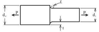
A model of this stepped shaft without relief groove is created using a student version of the ANSYS Parametric Design Language (APDL), Ansys, Inc., (2016), so that stresses at the aforementioned point can be found for various loading cases, i.e., various values of the ratio d _o / d _i . . A comparison is performed between the FEM - based value of the stress concentration factor and its theoretical value given after Equation (1) to (5), according to ^{Pilkey (1997)} for validation purposes.

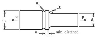
Next, another model of the stepped shaft is created using the APDL, this time including a relief groove, as shown in Figure 2. The radius of the groove and its position with respect to a specified minimum distance from the shoulder, are identified as u ₁ , u ₂ , respectively. The introduction of this feature is expected to diminish the stress at the root of the fillet, and to improve fatigue life, with optimum values of the geometry.

Source: Authors

Figure 2 Scheme of shaft with relief groove. 

Formulation of the optimization problem

The size optimization problem can be expressed as finding the set of design variables {u} that minimize the objective function, i. e., the maximum axial stress at both, the root of the shoulder fillet and the root of the relief groove, Equations (6), (7), (8), while subjected to the constraints given by Equation (9), ^{Pérez López (2002}).

The optimization problem is solved using an in - house tool, developed in MATLAB^®, applying the available optimization function fminimax, which minimizes the largest value of a set of multivariable functions, also known as the minimax problem, through the Sequential Quadratic Programming (SQP) algorithm.

Stress values to be minimized are not explicit functions of the design variables, u ₁ , u ₂ ; instead, stresses are parametrically calculated by the models built using the ANSYS Parametric Design Language, and their values are retrieved and updated by the optimization function. A proper interface between MATLAB^® and ANSYS is established, following a procedure set in ^{Gauchía et al. (2014)}.

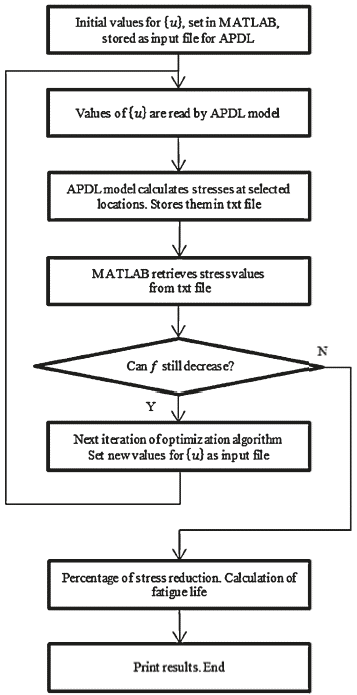
The flowchart of the implemented optimization approach is illustrated in Figure 3. MATLAB® sets initial values for {u}, stores these values in an input file (*.inp), and requests ANSYS to run in batch mode. The APDL model reads the input file, calculates values of stress at specified nodes, i.e., at the root of the shoulder fillet, and at the root of the groove, and stores these values in a text file (*.txt), which the optimization function fminimax can invoke. New values for the design variables, u ₁ , u ₂ , are set, and stresses are updated until their maximum value at the aforementioned locations is minimized, and stresses at both locations reach the same value.

Source: Authors

Figure 3 Flowchart of the implemented optimization approach. 

Criterion for calculation of fatigue life

Upon completion of the optimization process and obtainment of values of stress at both, the root of the shoulder fillet and the root of the groove, the fatigue life of the stepped shaft with and without relief groove is calculated, and their values are compared. To this purpose, the fatigue criterion of Dang Van has been selected, given that it shows good agreement with experimental results. A complete explanation of this criterion can be found in Dang Van et al. (1989).

This criterion evaluates an equivalent stress resulting from the combination of mesoscopic shear and hydrostatic stresses, then makes a comparison against the fatigue limit in fully reversed torsion, t_-1, Equation (14). As a previous step to the calculation of mesoscopic stresses, it is mandatory the obtainment of quantities such as the components of the macroscopic stress tensor, σ _ij (t), hydrostatic stress, σ _Η (t), macroscopic deviatoric stress tensor, S _ij (t), along one loading cycle, Equations (10) and (11).

The calculation of the deviatoric local residual stress tensor is not a trivial task when dealing with multiaxial or non - proportional loads, although for uniaxial loads evaluation of Equations (12) and (13) simplifies. The value of , is as in Equation (15),

An in - house tool has been developed in MATLAB®, for the calculation of fatigue life using this criterion and Basquin's equation (16). Stress components for calculation of fatigue life are taken from the value of σ _max = σ _{22 max} , , assuming a ratio R =σ _min /σ _max =-1

Numerical examples

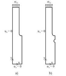
As a demonstration of the size optimization approach presented in this work, two parametric models of a stepped shaft subjected to an axial load were built. These models were both designed using the ANSYS Parametric Design Language as axisymmetric parts, using the element plane 183 and a mapped mesh. By using axisymmetry, only half the model was built, see Figures 4 a), 4 b). The models shown in these figures represent the shoulder filleted shaft without and with relief groove, respectively. The boundary conditions were, for both of them, left side, u _x = 0, bottom side, u _y = 0, top side, applied surface load. The number of elements, as well as their size, changed parametrically.

Source: Authors

Figure 4 a) Axisymmetric model of the shouldered shaft, without relief groove. b) Axisymmetric model of the shouldered shaft, with relief groove. 

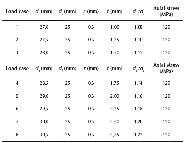
Both of them were subjected to eight loading cases, varying the maximum diameter, d _o , while keeping constant the values of the minimum diameter, d _i , fillet radius, r, and applied axial stress of 120MPa, thus creating various levels of stress concentration in the vicinity of the root of the shoulder fillet, see Table 1.

Table 1 Loading cases for eight values of the ratio d _o /d _i  

Source: Authors

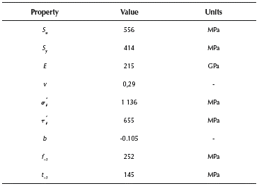
The material properties assigned for stress and fatigue life calculations were taken from 10HNAP steel, as referenced in ^{Kluger et al. (2004}), and they are listed in Table 2.

Table 2 Properties of 10HNAP Steel 

Source:^{Kluger, et al. (2004)}

Results and discussion

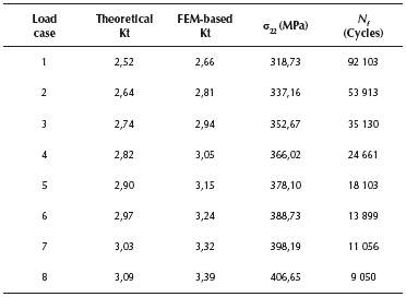
The model without relief groove in Figure 4 a) is loaded according with the cases listed in Table 1. Values of the stress concentration factor, defined as the ratio between the maximum stress at the root of the shoulder fillet and the nominal applied stress, are obtained using the finite element method through the APDL model. These values appear in Table 3, column 3, while the theoretical value of the stress concentration factor, by Equation (1), appears in Table 3, column 2. A comparison between finite element method based and theoretical values of the stress concentration factor is shown in Figure 5. The maximum axial stress at the root of the shoulder fillet and the fatigue life for this model, are seen in Table 3, columns 4 and 5.

Table 3 Maximum stress at the root of the shoulder fillet and fatigue life for the model without relief groove 

Source: Authors

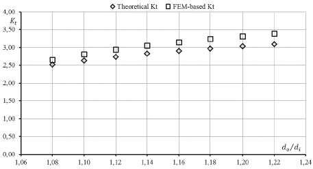
Figure 5 Theoretical and FEM - based values of the stress concentration factor for shafts without relief grooves. 

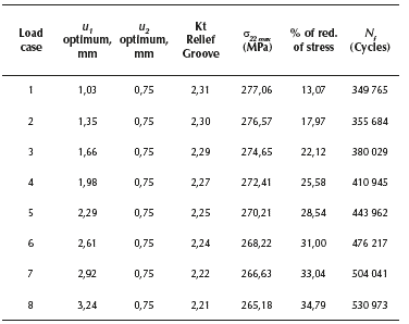
The model with relief groove in Figure 4 b) is also loaded according with the cases listed in Table 1. Optimum values of {u} that minimize the maximum stress at both, the root of the shoulder fillet and the root of the groove, are found for each loading case. Minimized values of stress are listed in Table 4, column 5.

In loading case 1, a percentage of reduction of stress of 13,07 % is achieved, for the model with relief groove, when compared against the model without relief groove. These percentages of reduction of stress achieved thanks to the effect of the relief grooves are reported in Table 4, column 6, for each one of the eight loading cases.

Table 4 Maximum stress at the root of the shoulder fillet and fatigue life for model with relief groove 

Source: Authors

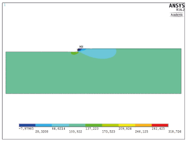
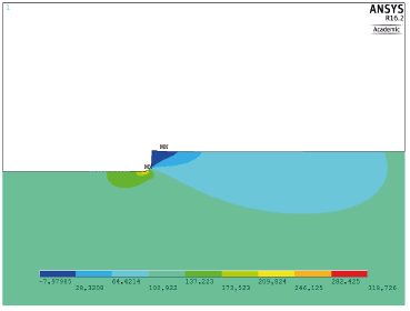
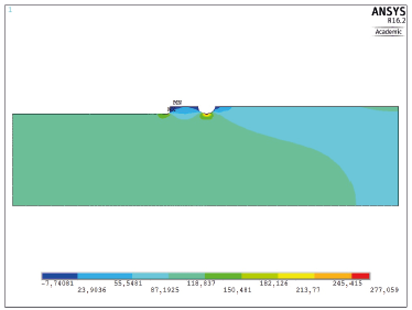
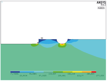
As for the improvement in fatigue life due to this design modification, in Table 4, column 7, values of N _f are listed for each loading case, considering a fully reversible load, using the Dang Van criterion. Figures 6 - 9 show comparisons between the stress distributions for the two models, loading case one.

Source: Authors, using Ansys Academic.

Figure 6 Stress distribution for model without relief groove. Loading case 1. 

Source: Authors, using Ansys Academic

Figure 7 Model without relief groove, case 1. Stress at the root of the fillet: 318,72 MPa. 

Source: Authors, using Ansys Academic.

Figure 8 Stress distribution for model with relief groove. Loading case 1. 

Source: Authors, using Ansys Academic.

Figure 9 Model with relief groove, case 1. Stress at the root of the fi llet and root of the groove: 277,05 MPa. 

According with Table 4, column 6, percentages of reduction of stress between 13 % and 34 % are achieved thanks to the introduction of the optimized relief groove. Fatigue life according with the Dang Van criterion and Basquin's equation has been calculated, for the stepped shaft with and without relief groove. These results are reported in Table 3, column 5 and Table 4, column 7. An improvement in fatigue life of the shaft is observed for the eight loading cases, ranging from a factor of 3,7 in loading case 1 up to a factor of 58,6 in loading case 8. This variation is due to the fact that the number of cycles to failure is calculated using a linear relationship on a log-log scale.

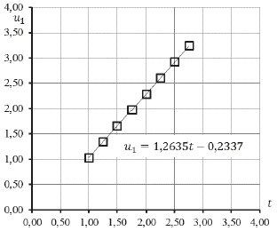
Optimum values of the design variables are shown in Table 4, columns 2, 3. Figure 10 would suggest a relationship between t (see Figure 1), and the optimum value of u ₁ (radius of groove), for values of d _o / d _i from 1,08 to 1,22, and for the applied loads and materials. This relationship could be expressed by Equation (17). Nevertheless, in order to express a general relationship between t and u ₁ for design purposes, a broader set of data ought to be analyzed.

Source: Authors

Figure 10 Relationshipbetween t and u ₁ for values of d _o /d _i from 1,08 to 1,22. 

Conclusions

Few studies have been devoted to the definition of the optimum geometry of relief grooves, when applied to shoulder filleted shafts in order to improve fatigue lives; therefore, an approach has been presented, aimed at minimizing the maximum axial stress at two points: the root of the shoulder fillet and the root of the relief groove on a stepped shaft subject to axial stress.

This approach is based on the use of an in - house developed tool working with the SQP optimization algorithm within the fminimax function, and which in turn, interfaces with a parametric model for stress calculations. Finally, fatigue lives of the shaft with and without relief grooves are calculated and compared.

Percentages of reduction of stress in the range of 13 °% to 34 °% are achieved for values of d /d. from 1,08 to 1,22.

This slight change in design also causes an important improvement in fatigue life.

The novelty of the approach lies in the inclusion of an optimization algorithm for the determination of the optimum geometry of relief grooves, using an interface between MATLAB® and ANSYS.

Results are encouraging since this approach can lead to the optimization of shafts featuring various stress relieving methods, or subjected to multiaxial loads. Further developments and the application of this methodology to practical design cases must include the appropriate safety factors.

Nomenclature

u _i , u ₂ - Design variables

K _t - Stress concentration factor

- Equivalent stress, Dang Van criterion

τ _f - Fatigue strength coefficient in shear

b - Fatigue strength exponent

S _u - Ultimate strength

f _-1 - Fatigue limit in fully reverse bending

t _-1 - Fatigue limit in fully reverse torsion

σ _ij .. - Macroscopic stress tensor

σ _Η - Hydrostatic stress

S _ij - Macroscopic deviatoric stress tenso

- Deviatoric local residual stress tensor

S _ij - Mesoscopic deviatoric stress tensor

N _f - Fatigue life, number of cycles

R - Stress ratio