Introduction

Among the non- destructive methods developed for the structural health monitoring (SHM) of structures and mechanical systems, the method based on electromechanical impedance (EMI) is particularly strategic due to its ability to detect minor structural damage, providing timely data for intervention (^{Giurgiutiu, 2014}).

Damage detection through EMI data is a crucial aspect in the practical application of this technique. To address this issue, various approaches have been devised to enhance damage detection using EMI technology, as demonstrated by ^{Kim and Wang (2019)}, ^{Fan and Li (2020)}, ^{Zhou et al. (2021)}, ^{Wang et al. (2022)}, and Nguyen et al. (2023).

Machine learning (ML) approaches for damage detection have yielded promising outcomes across various scenarios, with research endeavors delving into both supervised and unsupervised methods to unravel and leverage their potential. Specifically, in the realm of supervised ML techniques for damage detection, the predominantly employed algorithms center around neural networks, notably convolutional neural networks (CNNs) (^{Oliveira et al., 2018a}; ^{Rezende et al., 2020}, ^{Li et al., 2021}; ^{Ai and Cheng, 2023}; ^{Du et al., 2023}; Nguyen et al., 2023). Other noteworthy neural networks architectures include probabilistic neural networks (PNNs) (^{Na, 2021}), deep residual networks (DRN) (^{Alazzawi and Wang, 2021}), fuzzy ARTMAP networks (FAN) (Oliveira et al., 2018b), and extreme learning machines (ELMs) (^{Djemana et al., 2017}). These applications have demonstrated significant efficacy in classifying damage levels, often incorporating considerations for temperature variations.

Non- neural network- based supervised approaches include the random forest (RF) method, which was applied, among other techniques, by ^{Yan et al. (2022)} to monitor the early hydration of cement mortar, with promising results. Another application of the RF method developed for EMI- based monitoring was the prediction of impedance signatures in steel structures (^{Parida et al., 2023}).

In parallel, in the realm of unsupervised ML approaches, principal components analysis (PCA) has emerged as a pivotal tool in EMI- based monitoring. The method has found application as a damage index (^{Malinowski et al., 2021}) and has been employed for extracting crucial features from original impedance or admittance signatures (^{Park et al., 2008}; ^{Jiang et al., 2021b}; ^{Jiang et al., 2021c}; ^{Ai et al., 2022}).

In the context of the latter, PCA has been employed in conjunction with various complementary methods, including K- Means (KM) clustering (^{Park et al., 2008}; ^{Jiang et al., 2021b}), the support vector machine (SVM) method (^{Jiang et al., 2021c}), and artificial neural networks (ANN) (^{Ai et al., 2022}). These combined approaches have yielded promising results in EMI- based monitoring for damage detection.

Following the application of unsupervised methods in EMI- based monitoring, ^{Perera et al. (2019)} used hierarchical clustering and the KM method to detect damages in reinforced concrete (RC) beams.

PCA and KM show promise among the unsupervised methods used in EMI- based monitoring. However, there is a pressing need for more studies to explore the alternative applications of these techniques for effective damage detection. Moreover, the realm of supervised ML methods, including decision trees (DT) and RF, remains relatively uncharted or inadequately examined in EMI- based monitoring.

To address this research gap, our study offers a comprehensive comparative analysis of the KM, DT, and RF methods for damage detection using EMI signals, focusing on their capabilities in classifying four distinct structural conditions and utilizing two types of datasets: unprocessed raw impedance signatures and PCA- compressed datasets. Additionally, the study delves into the impact of dimension reduction on the models' efficacy in predicting damage occurrences.

To the authors' knowledge, the combined study of the DT and RF methods with EMI measurements for damage detection is limited or nonexistent. Hence, this work introduces a novel perspective, wherein the application of these methods can offer fresh insights into approaches for EMI- based damage detection.

Theoretical background

This section presents the theoretical concepts underlying the EMI method, followed by information on the supervised and unsupervised ML methods used to improve damage detection in this work.

Materials and methods

The experimental setup consisted of (i) an aluminum beam; (ii) a PZT patch; (ii) an Analog Devices AD5933 acquisition board; and (iv) a personal computer. The first step was to glue the PZT patch to the 300 x 25 x 3 mm aluminum beam (Figure 1).

Source: Authors

Figure 1. Aluminum beam and PZT patch used in the experiments 

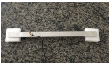
The procedure for gluing the PZT patch to the structure was of great importance. Since the impedance measurement was systemic (i.e., a measurement of the electro- mechanical impedance of the structure plus the PZT patch), it was essential to ensure a thin layer that was sufficient for the adhesion of the two surfaces and was not thick enough to induce other unwanted mechanical behaviors (^{Islam and Huang, 2014}; ^{Albakri and Tarazaga, 2017}; ^{Bari and Moharana, 2024}).

This gluing procedure consisted of applying a thin layer of epoxy resin onto the PZT patch and mounting it onto the surface of the specimen. Next, a thin 2 mm layer of EVA foam (ethylene vinyl acetate) and a weight of 1 kg were placed to ensure the homogeneity of the cure for the glue layer.

As the technique used was a differential and not an absolute procedure, i.e., the damage metrics were calculated concerning the reference integrity state, the effect of variations in the glue layer was disregarded.

Using wires, the PZT patch was connected to the AD5933 acquisition board to obtain the impedance signatures. The signal gathered from the AD5933 was read by the acquisition board's software on the personal computer.

The real part of an electrical impedance is known as the resistance (R), and the imaginary part is the reactance (X). Resistance represents the opposition to the flow of electrical current due to factors such as the resistance of conductors, circuit components, and, in this experiment, the mechanical movement of the structure. Reactance represents the opposition to the flow of current which arises from reactive elements such as capacitors (capacitive reactance) and inductors (inductive reactance). In this experiment, the reactance is capacitive because of the PZT patch. Electrical impedance is then represented as a combination of these two terms, where the real part is directly associated with the mechanical properties of the studied specimen.

In this work, the resistance was employed since it is the most sensitive to the presence of damage and is less affected by environmental conditions (^{Na and Lee, 2013}; ^{Hamzeloo et al., 2020}; ^{Meher et al., 2022}).

The acquisition system was set to cover a frequency interval varying from 60 to 70.2 kHz in steps of 20 Hz, resulting in 511 points in the frequency domain. The selected frequency interval was determined through trial and error, as it exhibited a high degree of sensitivity to the damage being assessed. Additionally, the interval range was selected to accommodate the resolution limitations of the AD5933 acquisition board.

The experiment involved four scenarios: one with the beam in its original state (baseline) and three others with damage. The damage was simulated by attaching a 10 x 10 x 10 mm magnet to the beam's surface in three different positions. The first damage position (Damage 1) was far from the PZT patch, whereas, in the subsequent scenarios (Damage 2 and Damage 3), the magnet was gradually brought closer to the PZT patch. For each scenario, 30 samples were collected, based on an average of 20 measurements in order to reduce random variation.

The collected data were analyzed in Microsoft's Visual Studio Code using the Python language (version 3.8.17). The datasets for each condition (Healthy State, Damage 1, Damage 2, and Damage 3) were imported using the Scipy package (^{Virtanen et al., 2020}) and consisted of two matrices. One dataset was related to the frequency data, which was presented as a one- row, 511- column vector, making it a vector of the frequency values, and the other corresponded to the real- part values of the impedance, with 30 rows and 511 columns, where each row represented a sample. Each column corresponded to a point within the frequency range in both datasets.

From the imported data set, the median of the resistance values along the frequency domain was calculated for the baseline condition and the three damage states, aiming to analyze the damage- related variations in the impedance signatures. All numerical calculations were performed using the Numpy package (^{Harris et al., 2020}), and plotting was performed using Matplotlib (^{Caswell et al., 2023}).

In the sequence, all the resistance matrices, each with 30 rows and 511 columns, were merged into a single one by concatenating rows, resulting in a 120- row, 511- column matrix. The first 30 rows were attributed to the healthy condition, the next 30 to Damage 1, and so on. The resistance values were then normalized to an interval between 0 and 1 to avoid undesirable effects caused by outliers once these signatures had been characterized by the presence of peaks, which could lead to significant differences in the magnitude of the values.

A one- row, 511- column vector of labels was created for each condition. The number 0 was assigned to the pristine condition, number 1 to Damage 1, and so on. The vectors containing the labels were merged using the same process employed for the real- part matrices of the impedance, resulting in a 4- row, 511- column matrix.

The resulting dataset was split into two parts, 70.0% for training the model and 30% for testing, in order to verify the models' ability to correctly predict the classes, which were all previously known: one baseline condition and three different damage levels. The dataset was partitioned using the Scikit- learn package (^{Pedregosa et al., 2011}).

The training dataset was used to obtain predictive models based on the KM, DT, and RF algorithms of the Scikit- learn package (^{Pedregosa et al., 2011}). In this step, the training data were based on the raw signature dataset of 511 variables.

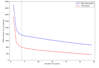
In determining the KM model, the number of clusters was an important parameter. Based on the Elbow method, this number was set to 4, and it was selected as the first point from which there were no significant changes in the within- cluster sum of squares (WCSS).

The models based on the DT and RF methods were created using entropy, i.e., Equation (1), as a criterion for defining the nodes, as well as based on the p(X) value, which is a fraction of examples belonging to a given class. Entropy is a measure of the purity of a group, wherein low values indicate high homogeneity or a high level of purity, and higher values indicate a lower level of purity.

The ability of the models to correctly predict the classes was determined by using the test dataset and submitting these values to the model. Accuracy, i.e., Equation (2), was used as a parameter to quantify the capability of each model.

Accuracy corresponds to the mean of the correctly predicted classes, where y is the actual class, and ŷ is the predicted class (^{Géron, 2019}; ^{Scikit- Learn Team, 2023}). This verification is performed along the test vector, which refers to the number of samples evaluated (n). The total number of times that the true values are equal to the corresponding predicted ones is divided by the total number of items in the test vector, resulting in an accuracy value.

The number of variables was decreased using PCA to evaluate the effect of reducing the dimensionality of the dataset on the models' ability to predict the classes correctly.

The PCA was selected over other dimensionality reduction techniques such as multidimensional scaling (MDS), uniform manifold approximation and projection (UMAP), and t- distributed stochastic neighbor embedding (t- SNE), given its simplicity and computational processing capabilities when dealing with data in high dimensions. Additionally, the PCA is less susceptible to the influence of outliers.

Moreover, the PCA method exhibits superior computational efficiency (it is a low complexity, covariance matrix- based linear method) when compared to nonlinear approaches. While the dataset utilized in this study may not be extensive, thereby yielding similar processing times across various dimensionality reduction methodologies, it is crucial to recognize that, within an automated system operating at scale and encompassing diverse structural configurations and sensor arrays over extended durations, this efficiency advantage can yield tangible reductions in energy consumption and decision- making times.

In this sense, the original training and testing data were transformed into principal components and used in the KM, DT, and RF algorithms.

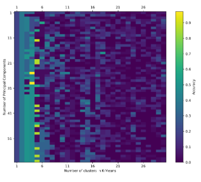
To build the KM model with the number of principal components and clusters, a routine was defined to obtain the optimal combination of parameters to maximize the model's accuracy.

Figure 2 shows the accuracy values for each tested combination. The results show that the highest accuracy value corresponds to 25 principal components and four clusters.

Source: Authors

Figure 2. Matrix chart of the accuracy values as a function of the number of principal components and clusters 

The execution of KM clustering -- and the other methods -- using the raw data and PCA information resulted in two prediction models, the first of which was based on 511 variables and the other on 25 variables (PCAs), with the latter representing a reduction of 95.1% in the number of features to be analyzed.

To allow for comparisons between the ML methods, the dataset consisting of 25 principal components was used to train the DT and RF models. Entropy was also used as a criterion to define the groups, and the parameters were the same as those used in the other models.

The resulting models were tested using the test set (30.0% of the data). Accuracy was also used as a parameter to quantify the models' ability to correctly predict the classes, and the results were used to make comparisons between the studied approaches.

Results and discussion

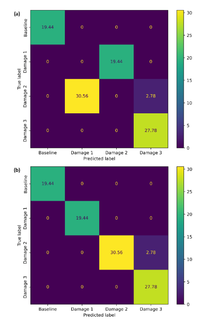
The analysis of the predictions generated by the KM models (Figure 3) reveals a notable discrepancy in performance. Specifically, the KM model relying on raw data exhibits many inaccuracies, as depicted in Figure 3a. This discrepancy is particularly pronounced for the first and second damage scenarios, wherein all predictions were erroneously classified. Conversely, accurate predictions were achieved for the baseline condition and the third damage scenario.

Source: Authors

Figure 3. Confusion matrix for the KM clustering models based on raw data (a) and PCA information (b) 

Figure 3 also shows that the same portion of the third damage scenario was misclassified as the second class, which may be due to the characteristics of the database itself -- probably the number of samples.

The PCA method's improvement in the classification ability of the KM algorithm can also be observed in the WCSS results (Figure 4). Considering the four clusters used, the WCSS for the PCA- based approach was 48.7% lower than that attributed to the raw data- based KM model.

Source: Authors

Figure 4. Plot of the WCSS obtained for the KM method using raw data and PCA information 

WCSS values indicate how compact clusters are, wherein high values reflect a high variability within the cluster. In this sense, the lower values obtained by the model based on principal components reflect a better classification.

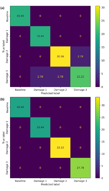
The results obtained with the DT method (Figure 5) show that the model based on the raw signature database yielded predictions that agreed with the corresponding true values (Figure 5a). Misclassification occurred in the second and third damage scenarios, with only small proportions of incorrect predictions.

Furthermore, misclassification occurred mainly between consecutive damage scenarios, probably due to the small differences between impedance signatures. The exception was the 2.78% of the third damage scenario that was misclassified as Damage 1.

Source: Authors

Figure 5. Confusion matrix for the DT models based on raw data (a) and PCA information (b) 

The results obtained via the DT model based on PCA information (Figure 5b) showed that all predictions matched the corresponding accurate labels, achieving a hit rate of 100%. Therefore, this model could differentiate all damaged scenarios based only on impedance signatures.

When comparing the raw data and the PCA- based results of the DT method, only a slight improvement was observed on one occasion. Even in the model based on the raw data, it was possible to obtain reliable results, with little deviations. This indicates that the DT method is a reliable and robust option when classifying structural conditions based on impedance signatures.

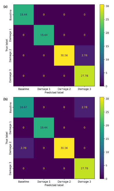
The confusion matrices obtained from the RF method are shown in Figure 6. The results show that the model based on raw data yielded predictions with minor deviations from the actual labels (Figure 6a), with only 2.78% of the third damage scenario misclassified.

Source: Authors

Figure 6. Confusion matrix for the RF models based on raw data (a) and PCA information (b) 

The results of the PCA- based RF model (Figure 6b) show a slightly higher deviation than that based on raw data, which may be due to the fact that the method is characterized as an ensemble. This feature can be better explored when dealing with large data.

However, the misclassification reported by the PCA- based RF model was only 2.78% higher than the results based on raw data, so the former does not represent significant changes concerning the latter. In this sense, the model based on PCA information can provide reliable results.

The accuracy obtained by each model (Figure 7) shows that KM clustering was the most sensitive to the dimensionality reduction of the dataset. In this case, reducing the number of variables from 511 to 25 principal components resulted in a 105.9% increase in accuracy.

Source: Authors

Figure 7. Accuracy results for each method in the two scenarios considered 

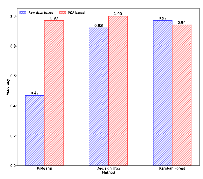
On the other hand, the DT method reported an improvement of only 9.1% when comparing the PCA- based results with the raw data- based ones, and the RF method showed a 2.9% decrease in accuracy when using PCA information. This behavior can be explained by the characteristics of the RF method, which can be advantageous in situations with a large number of variables.

When it came to using raw data for model training, the RF method yielded the best results and the KM model the worst. When the PCA data set was used, the DT method performed the best, correctly classifying all classes.

The KM method utilizing PCA compression outperformed the probability neural network (PNN) (^{Na, 2021}), which achieved an accuracy rate of 94.4%. Furthermore, the KM approach exhibited comparable outcomes to the CNN technique (^{de Rezende et al., 2020}), which reported a minimum accuracy rate of 97%.

The DT method showed the highest level of accuracy when using PCA information. It outperformed the PNN (^{Na, 2021}) and CNN (^{de Rezende et al., 2021}; ^{Du et al., 2023}) approaches and was comparable to other cutting- edge ML techniques for damage detection (^{Alazzawi and Wang, 2021}; ^{Jiang et al. 2021a}; ^{Ai and Cheng, 2023}). Additionally, the DT method utilizing PCA compression yielded superior results compared to the DT- based approach presented by ^{Jiang et al. (2021a)}, making it a noteworthy strategy for detecting damage using EMI data.

The results obtained with the RF approach were either comparable to or better than those obtained from the PNN method (^{Na, 2021}). Additionally, they closely matched the outcomes of other related studies (^{de Rezende et al., 2020}; ^{Jiang et al., 2021a}). Therefore, the RF method is a viable means to detect damage accurately. Moreover, it employs a single- step process and does not necessitate PCA compression to enhance the model's capabilities.

The results obtained herein show that reducing the number of variables generally entails an increase in accuracy, except for the RF method, without invalidating the use of the model.

The evaluation shows that the DT and RF methods are the most appropriate for damage detection in SHM applications using only a dataset of impedance signatures. When using PCA information, the former showed the highest accuracy, and the latter was the most stable, with acceptable accuracy values.

Conclusions

Identifying the presence of damage is a critical task in SHM systems. When using the EMI technique, the information derived from the impedance signature aids in detecting damage. When considering real- world applications, it is necessary to use adaptable techniques to provide reliable results in general situations.

This work used a dataset with impedance signatures of four classes in the KM, DT, and RF methods. In addition, to study the effect of reducing dataset dimensionality, PCA was applied, resulting in two scenarios for each method (i.e., raw data- and PCA- based).

The results show that, in general, reducing the number of variables in the model through PCA caused an increase in the accuracy of the models, with an exception attributed to the RF model. However, the decrease was not pronounced in this case, and the accuracy obtained was acceptable.

An analysis of the results showed the DT and RF methods to be the most suitable methods for damage detection based only on an impedance signature dataset. The former exhibited the highest accuracy value and good stability, resulting in a close and acceptable accuracy. On the other hand, the KM method managed to provide reliable results only by applying PCA to reduce dimensionality.

In addition, the approaches based on the DT and RF methods yielded results comparable to or better than other state- of- the- art solutions for damage detection using EMI.

According to the results obtained, applying supervised or unsupervised ML techniques for damage detection using EMI yields promising outcomes. Based only on a dataset of impedance signatures, an accurate classification was possible. Furthermore, by using the DT method, it was possible to achieve an accuracy of 100%.

The methods used herein are attractive options when it comes to damage detection using EMI data. Furthermore, the studied approaches do not require any pre- processing step before establishing the models.

In the experimental procedures, damage of the same severity was induced at varying distances from the PZT patch. Other works conducted by the authors have explored scenarios involving defects of different severity levels at the same distance from the patch. This proposal only considered the first scenario to check for feasibility, but different ML model responses for discerning different damage levels can be further explored.

Additionally, future research may focus on considering scenarios with different temperatures to enhance the use of unsupervised techniques for damage detection, bringing the approaches used herein closer to shop- floor industrial applications.