


 English (pdf)
 Article in xml format
 Article references

 Automatic translation
 Send this article by e-mail
 Cited by SciELO
 Cited by Google
 Similars in
SciELO
 Similars in Google

 Permalink


Introduction
Today, the world is facing the effects of climate change and other situations associated with it. That is the reason why countries are working hard to reduce the consumption of fossil fuels that generate more greenhouse gas emissions. By 2019, fossil fuels accounted for more than 80% of the global energy consumption. From this perspective, a considerable replacement of these fuels is expected to have been achieved by the middle of the century. For this purpose, implementing energy generation processes from renewable sources has been fostered to promote this transition to cleaner and more sustainable energies such as wind, solar, geothermal, and hydroelectric energy, among others 1.
In this regard, hydroelectric power generation includes hydroelectric and hydrokinetic turbines, being hydrokinetic turbines well accepted. These latter allow the use of a renewable source, like watercourses from rivers, seas, or artificial channels, to operate and produce energy. Hydrokinetic turbines take the kinetic energy of those sources and avoid the use of big-scale constructions, since they do not need a dam nor high altitude to operate. In addition, these turbines can capture energy without causing any significant disruption to the water stream, which means a low environmental impact. Additionally, it has been highlighted that these turbines are becoming very attractive due to their high energy density and the relatively easy way to be located near remote areas2.
Two types of hydrokinetic turbines are commonly known. The former ones are vertical or cross-flow turbines, where the axis of the rotor is orthogonal to the water flow and parallel to the water surface. This configuration allows unidirectional rotation, even though the fluid flow is bidirectional, and is suitable for operation in shallow channels with variable water velocities and shallow streams with limited water flow1. However, this kind of turbine has disadvantages, including low efficiency and, given its low starting torque, the requirement of a mechanism to start-up1-3. On the other hand, horizontal or axial flow turbines have their axis parallel to the direction of the fluid flow. The advantage of these turbines is their self-starting capability and the active control by pitching the blades allowing them more flexibility in over-speed protection3.
Several horizontal turbines can be the Archimedes turbines in screw and spiral-shaped. In the literature, it has been observed that Archimedes screw turbines present a high efficiency of approximately 85% when used in micro-hydroelectric power plants like hydraulic turbines4.
In recent years, studies based on Archimedes screw turbines for hydrokinetic applications have been introduced, carrying out numerical studies to determine the geometrical parameters and their optimal values to achieve a more efficient turbine5. The turbine efficiency has also been assessed through experiments at a laboratory scale for low tip speed ratio (TSR) values to discern the coefficient of performance of this kind of turbine aiming at producing the efficiency curve of the hydrokinetic turbine, both in aligned and inclined configurations6.
On the other hand, the spiral turbine has been recently used to produce energy, taking the wind to be operated, in order to determine the effect of certain geometric parameters on the operation and efficiency of this type of turbine. An investigation has established the turbine design parameters from angular momentum conservation, and studied the behavior of the turbine blade7. Based on computational fluid dynamics (CFD) results, this study concluded that due to the greater pressure difference in the blade tip, more energy could be extracted from the outside of the blade.
Despite the characteristics of horizontal-axis hydrokinetic turbines, they have a disadvantage associated with the low energy density that can be obtained compared to the turbines of hydroelectric power plants. For this reason, carrying out studies to optimize the geometry of these turbines is of utmost importance to achieve greater efficiency and, therefore, a higher performance in the energy production process.
In the field related to turbine simulation, it is possible to identify in the literature that in turbo-machinery, the six degrees of freedom (6-DoF) user-defined function (UDF) method has been commonly used to analyze systems as cross-flow turbines 8-11, water wheel turbines 12 and open flume turbines 13. The 6-DoF approach has not been thoroughly investigated in hydrokinetic turbine rotor modeling. From the authors’ knowledge, only the work carried out by Wang and coworkers was found to report the 6-DoF model in the CFD simulation to evaluate the performance of a vertical-axis Darrieus turbine 14. Bouvant et al. report an interesting study on the geometrical optimization of Archimedes screw hydrokinetic turbine (ASHT) as a hydrokinetic turbine 5. The authors provided significant improvement on the topic by comparing the results obtained with those reported in the literature, especially on the methodology used for the optimization. CFD numerical simulations have been improved with respect to those proposed by Zitti et al.6, substituting the constant angular velocity assigned to the turbine with a specific and more realistic UDF function 6. Furthermore, CFD results are extended with the use of response surface methodology. This leads to the identification of an optimal configuration compared with other CFD and experimental tests. For the numerical simulation, Zitti et al. applied the multiple reference frames (MRF) method in the ANSYS Fluent software6. The MRF method does not consider the inertia of the rotor, while it is considered by the 6-DoF UDF method that is utilized in the current research. Under this scenario, the presented work studies for the first time the hydrodynamic performance of an Archimedes spiral turbine (AST) for hydrokinetic applications.
In this work, a comparative study of the hydrodynamic performance of an AST and an ASHT was carried out. For this purpose, unsteady CFD simulations with the 6-DOF solver and the k-( shear stress transport turbulence model were employed. From the simulations, the power coefficient (Cp) curve for the AST was obtained and compared with the Cp curve of the ASHT that is available in the literature. The results calculated from the CFD method for the AST were compared with the experimental study reported for wind applications.
Methods and materials
The AST has a simple design, operates at low noise, and is environmentally friendly, with low-cost installation and maintenance associated. Its performance can be estimated in terms of Cp, which is defined as the ratio between the utilized power and the available power; i.e., the kinetic energy of the water is converted into rotational kinetic energy.
Cp is calculated from Equation (1) and depends on the TSR value; therefore, curves were obtained showing the values of Cp versus (vs.) TSR, being TSR calculated as expressed in Equation (2) .
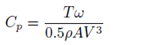
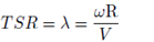
where T is the torque generated by the turbine, ω is the angular velocity, ρ is the density of the fluid, A is the swept area of the turbine, V is the fluid velocity and R is the radius of the peripheral section of the turbine.
AST has been studied by a number of authors for wind applications. For example, the behavior of the turbine has been compared for several blade inclination angles (() with respect to the axial axis. ( was fixed at several values, such as 50°, 55°, 60° and 65° (15). In this case, the higher Cp was equal to 0.22 at a TSR of 1.71 with a ( of 50°. Labib and coworkers concluded that higher Cp values were found at low TSR. In addition, a study has been conducted comparing the behavior of two different AST values (16). One of the AST had fixed angle blades (equal to 60°) and the other one had variable angle blades (equivalent to 30°, 45° and 60°). To study such as behavior, simulations were made in CFD. Finally, it was obtained that the maximum Cp (0.226) for the variable angle rotor was produced at a TSR equal to 1.96; while the maximum Cp reached for the turbine with a fixed angle equal to 0.207 occurs at a TSR of 1.57, resulting in a difference of only 9.18% compared to the maximum Cp of the turbine with a variable angle. Additionally, the referred authors indicated that the first and third blades of the turbine develop a key role in the extraction of energy, which in this case is wind energy (15).
Based on the previous information, some geometric parameters were established as conditions to be studied in the performance of an AST for hydrokinetic applications. Therefore, the spiral screw had three blades that were separated 120° between them. The turbine was defined by an outer diameter (De), a pitch (p) and ( equal to 250 mm, 170 mm and 60°, respectively. The geometry of the AST was similar to that used by Kim et al. (7) and Jang et al. (17). Figure 1 shows a schematic representation of the AST rotor model used in this study.
For the AST study, CFD simulations were implemented, employing the UDF, with 6-DOF, to model the rotation of the turbine. This solver uses the numerical integration of the pressure and the shear stress over the blade surface in order to compute the hydrodynamic force and moments acting on the blades. Additionally, the solver also keeps track of a rotor motion history, and post-processing the results, the angular velocity of the rotor is calculated from the force balance on the blade. In Equation (3), the translational movement for the center of mass of the body is calculated with respect to the inertial reference frame.
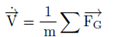
Where  ; m and
 refer to the translational motion for the body, the mass of the body and the vector of forces, respectively. In turn, Equation (4) was used to compute the rotation movement of the body, applying body coordinates; where
 is the vector of ω, L stands for the matrix with the inertia moments and
 is the moment vector of the object (ANSYS Inc., 2018a).

The 6-DoF approach can be used to predict sequentially the angular positions according to the turbine mass properties (mass and moment of inertia) in real time. The 6-DoF method computes the AST angular velocity (ω) based on forces and moments acting on the rotor.
For the 6-DoF simulation, the AST footprint and the entire domain were allocated in a way that with the water coming from -X to +X, the generated momentum would make the turbine rotates around the +X axis (one DoF rotation); the inertia tensor for the 6-DoF UDF configuration was computed with the help of SolidWorks software. The AST is limited to rotating around the X-axis, while the other DoF are not available. The specifications of the AST, which depend on the geometry and material of the turbine, are shown in Table 1. Small values of the moment of inertia promote the startup of the AST. However, excessively small values will impair the stability of the AST rotor rotation. For determining the moment of inertia, ABS (acrylonitrile butadiene styrene) was selected, and the material density was 1070 Kg/m3.
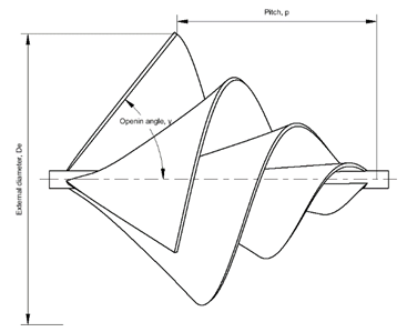
Table 1 Specification of the six degrees of freedom (6-DoF) body
| Parameter and units | Value |
|---|---|
| Mass [kg] | 2.70921 kg |
| Moment of inertia [kg·m²] | 0.00843 |
| Initial [rad/s] | 0 |
| Initial center of mass (x,y,z) [m] | (21.404, -0.012, -0.005) |
Once the configuration was completed, and the simulation was run, the 6-DoF model began to accelerate the body as a result of the interaction between the fluid and the turbine walls, and the ω rose to a stable and maximum value. From that point, a pre-load was set to the 6-DoF UDF and the turbine slowed down until the condition of 0 rad/s was reached. The preload of this study was 1.355 Nm. The collected data from the imposition of the pre-load allowed drawing the Cp vs. the TSR curve. As the simulation has only one rotational DoF, it was not necessary to employ any of the mesh methods found in the setup of dynamic mesh options of the Fluent software; this allows defining the rotation body as a rigid body whose rotational movement depends on the total momentum acting over the footprint surface. To ensure the correct transfer of information between the stationary and the moving domains, an interface boundary condition was employed, which also facilitated convergence.
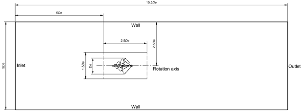
The computational domain illustrated in Figure 2 was similar to that employed by other studies in schemes concerning hydrokinetic turbines (5, 6). The fixed domain is a parallelepiped, while the rotational domain has a cylindrical shape. The dimensions of both of them are a function of De. The internal domain was located at 5 times De from the domain inlet.
The spiral-shaped turbine was modeled in the SolidWorks software, and the meshing was performed in the ANSYs Fluent meshing solver software. On the other hand, the three-dimensional (3D) unsteady simulation was carried out in ANSYs Fluent, where 3D Reynolds-averaged Navier-Stokes equations were solved with the k-( SST turbulence model. It is important to note that the k-( SST model is commonly utilized for hydrokinetic turbine modeling since it has been demonstrated to have better performance for complex flows, including adverse pressure gradients and flow separations, as occurs in horizontal-axis hydrokinetic turbines (5). The time step used for the simulation was 0.005 s.
In the domain, at the left surface, a constant velocity inlet equal to 1.2 m/s was applied. This velocity was considered as it is an average value in some important rivers in Colombia, such as the Magdalena or Cauca rivers, which have velocities between 1.1 and 2.5 m/s (18). In addition, in the right surface of the domain, a pressure outlet equal to 0 Pa was used. No-slip boundary conditions were applied at the surface of the blade. Wall boundary conditions were established in the other surfaces of the external domain. To ensure the correct transfer of information between the stationary and the moving domains, an interface boundary condition was employed, which also facilitated convergence.
During the numerical simulation, the quality of the generated mesh was checked by using the Richardson extrapolation. For this purpose, three different meshes were created and named as coarse, medium and fine mesh. The target parameter for the comparison of the meshes was the area under the curve formed by representing Cp vs. TSR. The Richardson extrapolation is based on Taylor’s series and allowed obtaining an improved estimate of the numerical result in derivatives, integrals, or differential equations (19).
The generalized Richardson extrapolation was well presented by Roache (1994) (20), standing a way to estimate the error associated with the spatial discretization in CFD simulations, which is considered one of the main numerical error sources. An additional and widely used concept is the grid convergence index (GCI) calculated between the size of meshes and the asymptotic range of convergence index (I), which brings an assessment of the discretization error among meshes. The values of I should be approximately 1 in order to ensure that the numerical simulation is within the asymptotic range (21).
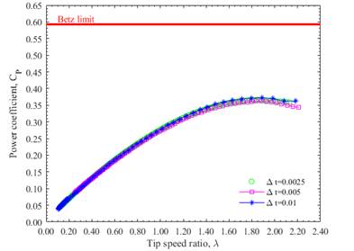
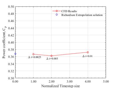
Figure 3 shows the results of the simulations (the evolution of Cp vs. TSR) carried out during the mesh independence test. For the number of elements used, the variation in the results due to the number of elements in the mesh can be observed to be not significant. In Figure 4, the asymptotic tendency of the results obtained with the used meshes is illustrated. This agrees with the value of I equal to 1.000054, which was obtained for the asymptotic convergence analysis. The  and
 values were 0.22% and 0.076%, respectively, showing that the grid independence was achieved. Thus, the medium mesh was selected for the simulations. The medium mesh was set at a first layer thickness of 1.58x10⁻³ m, a value that allowed obtaining a maximum dimensionless wall distance (y+) of 90.37, which is found in the range of 30 and 300, making it possible to use the wall functions approach 22.
Details for the different meshes are presented in Table 2. The meshes exhibited good quality parameters and the errors between the mesh results were less than 1%, which is also a good indicator of convergence. A representation of the medium mesh used in the numerical study is illustrated in Figure 5.
Both rotational and external domains were meshed employing poly-hex core mesh elements. The meshes of the rotational and fixed domains are illustrated in Figure 5.
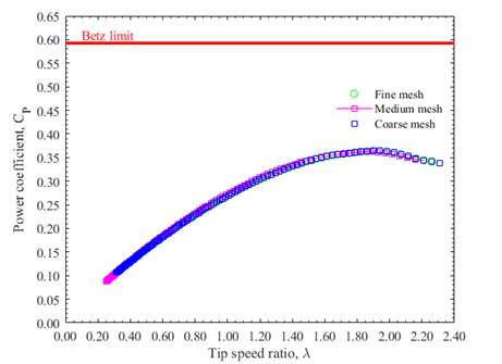
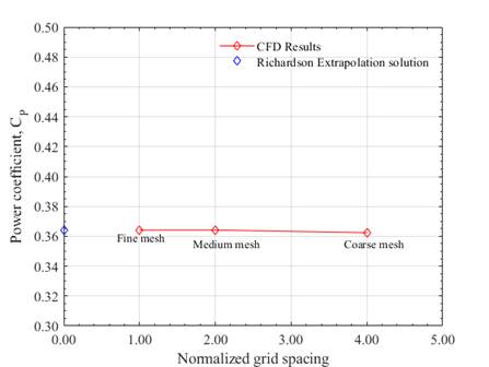
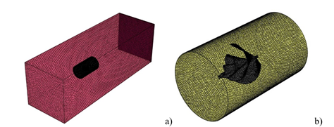
Table 2 Mesh independence test
| Parameter | Mesh | ||
|---|---|---|---|
| Coarse | Medium | Fine | |
| Number of nodes | 1866583 | 3907803 | 6537940 |
| Number of elements | 647898 | 1325345 | 2096639 |
| Max skewness | 0.699 | 0.699 | 0.699 |
| Mean aspect ratio | 3.156 | 2.885 | 2.814 |
| Min orthogonal quality | 0.301 | 0.301 | 0.301 |
As in the mesh independence study, the time step independency was developed by using 6-DoF simulations. The Richardson extrapolation process was adapted to analyze the time step influence on the simulation results; the test was carried out for three different time steps (0.00025 s, 0.0005 s, and 0.001 s) and in order to find the convergence time step index (CTI). The term CTI is the reciprocal of the GCI 23 and in this study, a value of 2% or less for the CTI was chosen as a criterion of selection for the definitive time step. The Cp vs. TSR curves for each of the above-mentioned time steps are represented in Figure 6. Little differences could be observed at the end of the curves; however, a good general concordance in the data behavior was also found. CTI12 and CTI23 were 1.69% and 2.28%, respectively; good results for CTI were noted in Figure 7, which covers a variation of less than 0.014. A time step of 0.0005 s was used in all the simulations. Additionally, when analyzing asymptotic convergence for the time step, a value of 0.9952 was obtained. This value is close enough to 1 to consider that the selected time step is in the asymptotic convergence region.
Although the criterion adopted to terminate the iterative process was based on the residual of the corresponding equation (e.g., the equation for the pressure), during the numerical analysis the convergence of the simulation was not assessed in terms of the achievement of a particular level of residual error. Solution-sensitive target quantities were carefully defined for the integrated global parameters of interest and an acceptable level of convergence was selected based on the rate of change of these values (e.g., Cp). The convergence criterion was set at 10-4 during all the simulations. For the CFD simulation, the first-order upwind scheme was used for the treatment of advective terms and PRESTO (Pressure Staggering Option) for the spatial discretization of pressure in the momentum equation. The couple scheme pressure-velocity was selected as the coupling algorithm and was adjusted through the PISO (Pressure Implicit Split Operator) algorithm.
Results and discussion
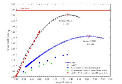
Figure 8 shows the ratio between Cp and TSR for the AST, which is obtained by the simulation, and the numerical and experimental results reported for an ASHT by Mael et al. (5. This turbine consists of a screw coupled to an electric generator and a support structure. Comparing the AST with the ASHT, the Cp value for the former was 0.3369 at a TSR equal to 1.909. On the other hand, the ASHT achieved a Cp of 0.5515 at a TSR equal to 1.35 5. The maximum Cp is slightly higher than those with similar AST presented in the literature for wind applications 15-17,24-26. It is evident that the Cp of the AST is lower than that of the ASHT. This can be ascribed to the fact that, although a good area of contact with the fluid is achieved with the spiral turbine, this is lower than the area provided by the traditional screw, resulting in a lower amount of energy extracted from the fluid. Furthermore, it was noticed that ω for the maximum Cp was 18.39 rad/s. A comparison between the CFD results of the AST for hydrokinetic applications and experimental data for wind applications at a flow velocity of 5 m/s was also represented in Figure 4 16. The geometry for the AST, whose experimental results were presented in Figure 8 16, was similar to that one evaluated in this study. In the figure, for wind applications, the Cp values were lower; however, the trend of the curve was similar.
The AST had a greater Cp at the lower TSR than the Savonius turbine, which makes the AST suitable for river currents with low and varying velocity. For Savonius hydrokinetic turbines, the typical maximum Cp is about 0.2 at a TSR between 0.7 and 0.8 27.
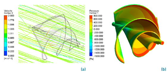
In addition, in Figure 9, the streamlines and pressure contours for AST are illustrated. It is observed that the velocity values in the streamlines are low at the inlet. This can be explained because the flow is not disturbed yet, but as it passes through the blades, this velocity increases, and then decreases at the turbine outlet. The AST operation depends on the use of both lift and drag forces. Nevertheless, the force causing the rotation of the blade dominantly is the drag acting on the three blades 17. Figure 9b shows the pressure distribution on the spiral. When the AST is rotating, there is a pressure difference between the pressure side and the suction side. Due to the spiral surface of the blades, the pressure difference generates torque. In general, the front side of the blade has a higher pressure while the corresponding rear side has a lower pressure. Figure 9b also shows that the location of the stagnation pressure region was near the leading edge and the helical blade tip. This means that most of the energy can be extracted near the blade tip like a three-bladed horizontal-axis hydrokinetic turbine.
According to the results informed for the ASHT 5, the authors indicated the influence of the helix angle and the diameter ratio on the Cp, pointing out that a low diameter ratio (inner diameter/outer diameter; i.e., Di/Do) leads to a larger blade area. In this regard, more energy can be extracted from the fluid. This allows observing that, in an AST, parameters such as ( have significant influence on the Cp. Therefore, in order to obtain an AST with the design parameters optimized for obtaining the highest performance, the turbine Cp is required to be improved.
Conclusions
In this study, the performance of an Archimedes spiral turbine (AST) for hydrokinetic applications was calculated by unsteady computational fluid dynamics (CFD) simulations. As a result of the numerical simulations, a maximum Cp of 0.3369 was observed when the tip speed ratio (TSR) of the rotor was 1.909. In the unsteady state simulation, when the water flow passed the blade, the flow needed to accelerate to pass the spiral surface of the blades. As the water continuously passed the AST blade, it created a low-pressure area on the tip of the blade because the water across this area had a higher velocity. The maximum pressure differences were observed at the blade tip, suggesting that the most kinetic energy could be extracted from the outer part of the blade. In order to improve the turbine Cp, further research focused on optimization techniques is needed to know the influence of each design parameter on the turbine performance.
It was also observed that the AST, as a hydrokinetic technology, has a high potential for power generation in remote areas due to its easy fabrication, installation, and good performance. However, experimental research is needed to discern the real behavior of the AST turbine under working conditions. The results of these investigations would allow validating the simulation methods used here and select the most suitable one for the study of this type of turbine.