




 English (pdf)
 Article in xml format
 Article references

 Automatic translation
 Send this article by e-mail
 Cited by SciELO
 Cited by Google
 Similars in
SciELO
 Similars in Google

 Permalink


Introduction
Landslides are among the most deadly natural hazards and cause large economic losses all over the world each year1-4. Approximately 5% of the total global population lives in landslide-prone areas5, and in countries such as the United States, Japan, Italy, and India, economic losses are estimated to be over $1 billion per year6. Between 2004 and 2010, an estimated 32,322 people lost their lives due to non-seismic landslides7.
Rainfall is the most common cause of landslides8-10 and is responsible for the highest number of casualties. Landslides triggered by rainfall account for 89.6% of landslide fatalities worldwide11. Based on the EM-DAT database from OFDA/CRED, a world annual average of 914 deaths were reported between 2005 and 2014 due to rainfall-related landslides 12.
One of the most frequent causes of natural disasters in the tropical and mountainous countries of the Circum-Pacific region are landslides triggered by rainfall 13-15. Colombia, located in the northern corner of South America, is characterized by tropical conditions and mountainous terrain16. The most important urban centers are located in the highlands and valleys of the Andes Mountains. Due to these natural conditions, Colombia has a long history of landslide disasters 17. A debris flow on November 13, 1985 devastated the city of Armero, killing approximately 22,000 people and causing economic losses totaling over $339 million18-20. In the city of Medellin on September 27, 1987, a mudslide with a volume of 20,000 m3 destroyed more than 80 houses and killed approximately 500 people21. More recently, on April 1, 2017, a total of 130 mm of torrential rains triggered several landslides in the mountainous terrains of the southern Colombian Andes, causing a flash flood and debris flow along the Mocoa, Sangoyaco, and Mulato rivers that destroyed 17 neighborhoods in the city of Mocoa that were built along the riverbanks. At least 314 people were killed, and an additional 106 people were missing22.
However, landslide impact assessments are often limited due to the scarcity of reliable observations, particularly in remote high-mountain regions such as the Colombian mountains. Data availability is one of the most important factors for analysis, assessment, and modeling of landslides triggered by rainfall. The areas affected by landslides are often remote and difficult to access. For this reason, the development of regional landslide susceptibility analysis has proven difficult in the locations where it is most needed23. Due to this lack of data in many regions, remote sensing data may be used for landslide susceptibility analysis, especially in developing countries24.
A landslide susceptibility assessment is critical for planning, sustainable development, and risk mitigation because it provides information on the likelihood of landslides occurring in an area given the local terrain conditions25. There are several methodologies to assess landslide susceptibility26. They are divided into qualitative or knowledge-driven methods and quantitative or data-driven methods. Knowledge-driven methods are based entirely on the judgment of the earth scientist, and the zoning baseline data is sourced directly from field visits26-29. The primary limitation of the qualitative method is that the accuracy depends on the knowledge of the experts. Data-driven methods are subdivided into deterministic and statistically based methods30-32. While deterministic methods assess slope failures using the factor of safety at large scales33 and require detailed information and parameters, statistical methods evaluate the relationship between landslides and causative factors to predict the occurrence probability through the use of GIS tools that reduce the subjectivity and biases in the process of weighting landslide causative factors. The widely used statistical methods are bivariate34-36, multivariate16,37-40, and neural networks41-43. Logistic regression (LR) is the most widely used multivariate statistical analysis method39,44-48. LR is independent of the data distribution and can be incorporated into the analysis of a variety of data sets, such as continuous, categorical, and binary data. However, the selection of landslide causative factors is significant for LR methods49,50. Irrelevant independent variables should be removed, and only optimal causative factors should be included in the analysis50,51.
This case study assesses the landslide susceptibility of a data-scarce study area in the Colombian Andes where, on May 18th, 2015, dozens of landslides were triggered by a rainstorm that caused a major debris flow and flash flood resulting in 104 deaths and economic losses not yet estimated. The study uses DEM, Google Earth images, orthophotos and aerial photography. To select the positive causative factors related to landslide occurrence and the model validation, the area under the ROC curve was applied.
Study Area
The Liboriana catchment is located on the northern side of the Western Cordillera in the Colombian Andes, approximately 500 km northwest of Bogota City (Figure 1). It lies between latitudes 5º55’30”N - 6º1’0”N and longitudes 75º58’W - 76º6’W, and covers an area of approximately 59 km2. Two populated areas, La Margarita village, and Salgar town, extend along the central and lower portion of the river valley and have a population of approximately 8,820 inhabitants.
The catchment has a tropical humid climate with a mean annual temperature of 22 °C. The maximum temperature occurs between February and April, while the minimum occurs between October and November. The precipitation regime is dominated by high variability at both inter-annual and inter-seasonal scales. The mean annual rainfall is 3,073 mm, and the monthly rainfall distributions show evident seasonal patterns with two rainy seasons, with rainfall peaks in May and October52,53.
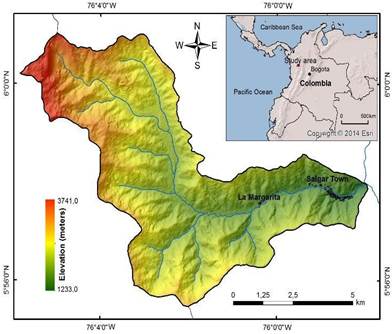
The geomorphology of the upper catchment consists of a mountainous region with a rugged morphology, narrow valleys, and very steep forested hillslopes. The elevation varies from 1233 to 3741 m a.s.l. with a mean of 2487 m a.s.l. The zones with slope gradients exceeding 30° account for 67% of the total area. The upper part of the catchment consists of deep forests, while the middle and lower zones contain grasslands and coffee plantations that have replaced the forest.
The Liboriana catchment is composed predominantly of a Cretaceous sedimentary rock formation (shales, limolites, sandstones, cherts, and conglomerates with some intercalations) and an intrusive Miocene body54,55. These rocks have been severely weathered in situ under the humid tropical climate, forming residual soils and saprolite.
The may 18th, 2015 rainstorm
On May 18th, 2015, heavy rains in the northern Colombian Andes caused a MORLE-type landslide (multiple-occurrence regional landslide event) (56 in the Liboriana catchment. Most of the individual landslides constituting this MORLE call event displaced all the regolith and left exposed rock. Due to the steep slope of the terrain, surficial rockslides also occurred. Large amounts of water and solid material were transported down to the primary river channel, causing a flash flood and a debris flow that swept away everything in its path, including La Margarita village and the lowest areas of Salgar Town. Authorities confirmed 104 deaths, 62 injured, and 1440 directly affected people. The flash flood and debris flow destroyed at least 66 houses and 6 local bridges . This is the fourth deadliest weather-related disaster in Colombia’s recorded history.
Reports from the SIATA weather radar (early warning system of the city of Medellin and the Aburrá Valley, in Spanish) indicate that between 10 pm on May 17th and 2 am on May 18th, a rain cell on the west side of the catchment at Cerro Plateado caused intense precipitation in approximately 30% of the total basin area (~20 km2). During this four-hour period, the total accumulated rainfall was 100 mm. Other minor rainfalls occurred until 7 pm on May 18th, for a total of 160 mm of rain that fell in the upper part of the basin in a 20-hour period.
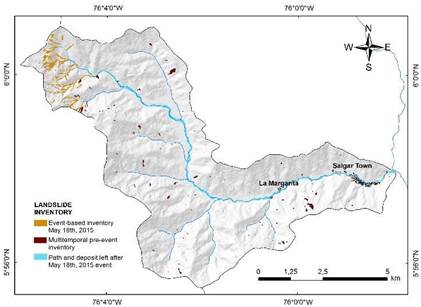
Google Earth provided free and open post-event satellite imagery to obtain the event landslide inventory and the flash flood path and area occupied by the debris flow (Figure 2). A total of 160 shallow landslides were triggered during the MORLE event from the May 18th, 2015 rainstorm; however, in the Liboriana catchment, a total of 50 associated landslides were identified.
Methodology
A wide range of quantitative methodologies are used for landslide susceptibility assessments34,57-60. Statistical methods estimate landslide probabilities based on the correlation analysis between causative factors and historical landslide occurrences.
Table 1 Combinations of the causative factors for the five different susceptibility models to apply LR
| Models | Included factors | Missing factors |
| M1 | Aspect, land cover, curvature, slope, TWI | |
| M2 | Land cover, curvature, slope, TWI | Aspect |
| M3 | Aspect, land cover, slope, TWI | Curvature |
| M4 | Aspect, land cover, curvature, slope | TWI |
| M5 | Aspect, land cover, slope | Curvature, TWI |
LR is one of the most frequently used multivariate statistical analysis models to predict landslide occurrence at medium and regional scales39,46,61. LR estimates the relationship between a dependent variable, measured with dichotomous values such as 0 and 1, and a set of independent terrain variables. The advantage of LR is that the prediction factors do not require normal distribution data and may be either categorical, non-categorical, or any combination of both types62. The dependency relationship between the landslide occurrence and the independent variables can be quantitatively expressed as:
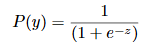

Where P(y) is the estimated spatial probability of the landslide occurrence and ranges from 0 to 1. z is the following linear combination of the independent factors:

where b0 is the intercept of the model given in the LR output, the bi values (i=1, 2, 3, …, n) are the regression coefficients, i.e., variable weights, and the xi values (i=1, 2, 3, …, n) are the independent factors. The final model is a LR based on the independent variables of the landslide occurrences (presence or absence).
The LR algorithm was applied to the landslide susceptibility assessment of the Liboriana catchment using the IBM Statistical Package for Social Science (SPSS) for five different causative factor combinations (Table 1).
To validate the accuracy and prediction capability of the models and to select the best susceptibility model, different validation methods were applied. The most common validation methods in landslide studies are threshold-independent approaches, especially the Receiver Operating Characteristic (ROC) analysis63,64. ROC analysis is based on the confusion matrix in which actual classes, called positive and negative class labels according to landslide inventory databases, are compared with the predictive classes, called true and false class labels, produced by the model63. Figure 3 shows the four possible outcomes of the confusion matrix. An advantage of ROC analysis is that several statistics have been defined for evaluating model performance and prediction, such as precision (PR) and accuracy (AR), among others. During the performance and prediction evaluation, the hit rate (TPR), false alarm rate (FPR), and odds ratio (OR) were calculated and used for a quantitative comparison.
The area under the ROC curve (AUC) is a useful indicator to validate the success rate when the landslide susceptibility map is tested against the landslide database used to train the model, and the prediction performance of the model when the landslide susceptibility map is tested against future landslides or a landslide database not used to train the model. The AUC value is between 0 and 1, and a higher value indicates a higher prediction success or prediction rate, whereas a value of 0.5 indicates that the prediction is no better than a random guess64.
In addition to this analysis, the distance to perfect classification (r) (65,66 and the degree of fit (D.F.) (67 were applied using the following equations:

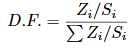
Where Z i is the area occupied by the rupture zones in the i class of susceptibility, and S i is the area of the i class of susceptibility.
Landslide inventory
Landslide inventories are the first and most important step in landslide susceptibility analysis using statistical methods23,64,68-70. In this study, landslide locations were determined using the 2015-updated Google Earth imagery, an open access 1:10,000 scale orthophoto from the period 2010-2012, and aerial photography from 1998 and 1999. As a result, a total of 259 landslides were collected (Figure 2). All the landslides cover an area of 0.56 km2 and account for approximately 0.95% of the catchment, of which 33% correspond to landslides triggered by the May 18th, 2015 rainstorm, and 67% correspond to multitemporal landslides with no time occurrence specification that occurred prior to the May 18th, 2015 event.
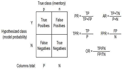
Table 2 Results of the different validation methods including the AUC-ROC model values for the success and prediction rate, the distance to perfect classification (r), and the ROC metrics hit rate, false alarm rate, and odds ratio
| Models | AUC ROC success rate (%) | AUC Prediction rate (%) | Distance to perfect classification (r) | Hit rate (TPR) (%) | False alarm rate (FPR) (%) | Odds ratio (OR) |
| M1 | 68.1 | 67.3 | 0.521 | 0.619 | 0.356 | 2.94 |
| M2 | 65.0 | 64.9 | 0.574 | 0.554 | 0.361 | 2.19 |
| M3 | 68.2 | 67.3 | 0.518 | 0.611 | 0.342 | 3.02 |
| M4 | 68.8 | 69.5 | 0.520 | 0.606 | 0.339 | 2.99 |
| M5 | 68.7 | 69.4 | 0.517 | 0.613 | 0.343 | 3.03 |
Considering the cross-validation method proposed by Chung & Fabbri64, the landslide inventory data was split into three groups: (i) the event-based landslide inventory of 50 landslides associated with the May 18th, 2015 rainstorm, which were used to perform a temporal validation of the landslide susceptibility map; (ii) the training dataset that corresponds to 80% of the randomly selected landslides of the multitemporal past landslide inventory to be used for building the LR model (167 landslides); and (iii) the spatial validation dataset that corresponds to the remaining 20% of the multitemporal past landslide inventory to be used for the spatial validation process (42 landslides).
In addition to the landslide areas, non-landslide areas are required to form the dichotomous variable to apply the LR method 69. In this study, non-landslide points were determined by randomly selecting the same number of pixels from the areas with no record of landslides.
Several mapping strategies are used to develop a landslide inventory map26,29,71. The spatial location of landslides can be represented by points in raster-based maps that correspond to the centroid of the entire landslide or the scarp area46,72-74, polygons that correspond to all the pixels within the entire landslide body or the scarp area28,44,64, and lines that correspond to the pixels of the upper edge of the landslide scarp area75,76. Several studies have indicated that the scarp is the best sampling strategy for the landslide susceptibility assessment77-79. In this study, the landslide scarp was used to represent pre-failure conditions, excluding both the transport and the deposition zones of existing landslides.
Landslide causative factors
The selection of the relevant causative factors is a fundamental step in the landslide susceptibility analysis because it improves the prediction accuracy28,50,69,80. In general, they must have a certain affinity with the dependent variable, they must be represented across the study area, and they have to be measurable and non-redundant44. In this study, based on data availability and topographical, hydrological, and geological catchment conditions, a total of 5 landslide predictor variables were initially used. They were divided into morphometric and environmental factors.
Morphometric factors
Morphometric attributes derived from digital elevation models (DEM) are increasingly used in landslide susceptibility assessments81. The available topographic maps (1:25,000 and 1:10.000 scales) only cover approximately 25% of the easternmost part of the study area. To obtain the morphometric attributes, a free access DEM was obtained from the Alaska Satellite Facility program82 with a spatial resolution of 12.5 m. This DEM was used to derive the aspect, curvature, slope gradient, and topographic wetness index (TWI) using ArcGIS 10.2 software (Figure 4). All these factors are related to landslides to a different degree.
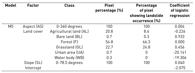
The relationship between the aspect and landslide occurrence has been widely studied(45, 61, 83). The slope aspect is related to the sunlight exposure and soil moisture conditions of the hillslopes48 (Figure 4a). The down-slope and across-slope curvature values were calculated and crossed to determine the total curvature according to Ayalew & Yamagishi 44 (Figure 4b). The profile curvature influences the driving and resisting stresses within a landslide in the direction of motion. It controls the change of velocity of a landslide flowing down the slope. In contrast, the plan curvature controls the convergence of landslide materials and water in the direction of the landslide motion. The slope angle is typically defined as the crucial landslide-conditioning factor because it controls the shear forces acting on the hillslopes. However, its relationship is not always proportional, and the maximum relative frequency of landslides typically corresponds to medium slope angles (Figure 4c) 48. Finally, TWI is a hydrological factor frequently used in landslide studies83-85 (Figure 4d). It is a function of the slope and the upstream contributing area per unit width orthogonal to the flow direction.
Environmental factors
In a tropical landslide-dominated zone such as the Liboriana River basin, land use is typically associated with landslide occurrence85,86. The available land use data consisted of only a 1:100,000 map, which is a very small scale for the purposes of this study. Thus, the data used were obtained primarily from Google Earth imagery and supported by the 2010-2012 orthophoto to produce a detailed map. The resulting layer in GIS includes six categorical values (Figure 4e): agricultural land, bare land, forest, grassland, urban area, and water body.
Although lithology is one of the essential conditioning factors in most of the landslide susceptibility analysis, approximately 90% of the total area in the Liboriana catchment corresponds to undifferentiated sedimentary rocks(54, 55). This geological homogeneity indicates that lithology does not explain the landslide distribution and spatial location.
Results
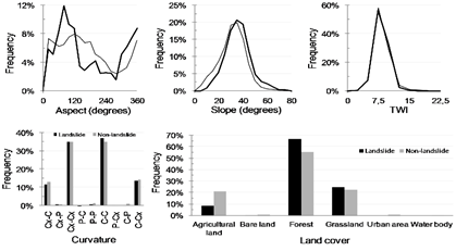
ta landslide and non-landslide group for each terrain and classified into intervals to plot the frequency distributions for the different causative factors (Figure 5). The slope, aspect, and land cover factors have a closer relationship with landslide occurrence because there is a significant difference between the landslide and non-landslide curves.
According to the slope aspect, the landslide frequency increases on east-facing and north-facing slopes. The correlation analysis between slope angle and landslide occurrence has a normal distribution. Gentle slopes have a low landslide frequency that increases with the slope gradient to reach a maximum value at approximately 40°, followed by a decrease in landslide frequency. Steep natural slopes resulting from outcropped bedrock are not typically susceptible to shallow landslides. Regarding the land cover, the results show that most landslides fall into the category of forest and grassland-covered areas. For the TWI and curvature, a difference is not observed between the landslide and non-landslide groups. For curvature, landslides typically occurred on horizontal and vertical concave or convex slopes. For the TWI factor, landslide frequency typically occurred at values of approximately 8.
LR was applied to the five susceptibility models shown in Table 1. The regression coefficients of the prediction factors were used to create the landslide susceptibility map for the five susceptibility models. Quantitative validation was conducted by comparing the five susceptibility maps with the landslide spatial distribution inventory. The training dataset was used for the success rate, and the spatial validation dataset was used for the prediction rate. The results were plotted in the ROC space with the ROC plots (Figure 6). The ROC curves show similar success and predictive capabilities for all the susceptibility models; only model 2 has a slightly lower value.
The distance to perfect classification (𝑟) was determined for every model with the TPR and FPR values using Equation 3.
Table 2 defines the statistics used in this study. The AUC-ROC values for all the models indicate an acceptable ability to distinguish between susceptible and non-susceptible landslide areas. The hit rate, also referred to as the sensitivity or positive accuracy, expresses the proportion of positive cases predicted correctly. The false alarm rate, also called the negative error, is the ratio between false positives and actual negatives. The odds ratio uses all the values in the confusion matrix because it shows the ratio between correctly and incorrectly classified observations.
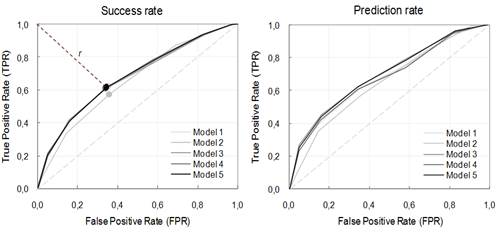
Figure 6 ROC success and prediction rate curves for each model, and distance to perfect classification (𝑟). The dotted line shows the shortest r-value, which corresponds to M5
According to the results, both M4 and M5 have an adequate and similar trend for the success and prediction rate. M4 is slightly better on the ROC plot (68.8% AUC). However, M5 has a shorter distance to perfect classification (0.517), and a slightly better value for the hit rate, false alarm rate, odd ratio, and frequency distribution curves (Figure 5).
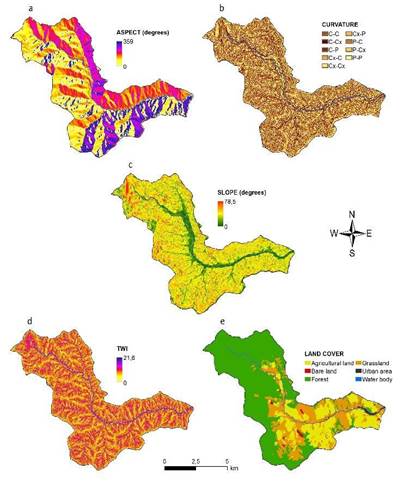
Table 3 shows the LR coefficients of the susceptibility model M5 that correlate each factor to the landslide occurrence. LR determines a coefficient for every non-categorical variable and a coefficient for every class of the categorical variables.
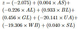
The probability of landslide occurrence was calculated by applying Equation 1 and Equation 2, which use the LR coefficient data in Table 3 and each variable raster. Equation 5 shows how Equation 2 was formulated for the M5 model.
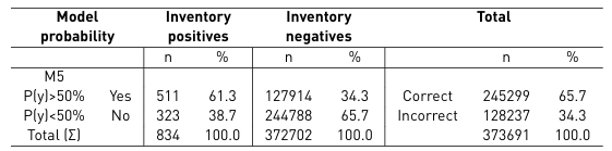
After building the model and determining a continuous response variable expressing the degree of susceptibility, a decision threshold (cutoff value) of P(y) = 50% was selected to classify the continuous response dependent variable as landslide (yes) or non-landslide (no). This value corresponds to the same inflection point of the ROC plot and the point with the lowest value for the distance to the perfect classification. Then, the confusion matrix was performed by comparing these predictions with the observations in the validation landslide inventory dataset. The results presented in Table 4 show the number of correctly and incorrectly predicted observations for both the positive and negative cases. The false positives, or error type I, correspond to 34.3%; conversely, 38.7% represents the false negatives, or error type II. The susceptibility model is more efficient at correctly classifying slopes absent of landslides and less efficient at classifying slopes that contain landslides.
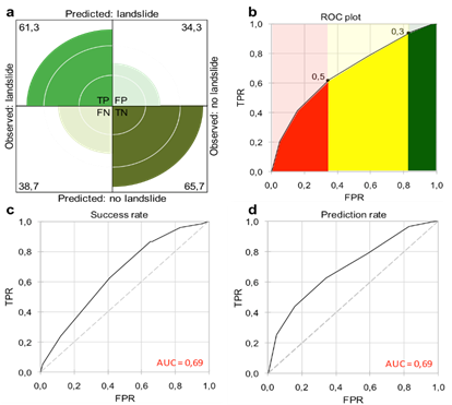
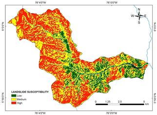
The susceptibility map of the M5 model is presented in Figure 8. The probability histogram was divided into the three susceptibility classes (Table 5). The upper limit of the medium class is the inflexion point of the ROC curve, which is the same point as the distance to the perfect classification (0.5). Additionally, the lower limit of the medium class is a subtle change in slope at 0.3 (Figure 7b). Figure 7 shows the primary graphical output and results determined from the validation phase for the M5 model. It includes the ROC plot success and prediction rates with the AUC value (Figures 7c and 7d) and a fourfold representation of the confusion matrix (Figure 7a).
According to the landslide susceptibility map acquired from the LR (Figure 8), 34.4% (20.1 km2) of the entire area was classified as highly susceptible, while approximately 48.4% (28.3 km2) was classified as a medium landslide susceptibility zone. The low susceptible zone contained 17.2% (10.0 km2) of the entire area.
High susceptibility zones have a landslide density of 25.7 landslides/km2, and 64.7% of the landslides triggered on May 18th, 2015 were in this susceptibility class. A total of 35.3% of the May 18th, 2015 landslides occurred in the medium susceptibility zone. Additionally, there are 4.9 landslides/km2 for the low susceptibility zone, and none were associated with the May 18th, 2015 event.
Table 4 Confusion matrix for M5; inventory positives are cells with landslides, negatives otherwise. These values are compared to P(y) (probability estimated by LR). The total correct and incorrect predicted cells are shown on the right
Discussion
During the last century in Colombia, the settlement expansions along the inter-Andean valleys have increased the risk to human lives and infrastructures and, consequently, the number of disasters with significant human loss. To identify the risk caused by landslides to human settlements and to minimize the loss of lives, it is fundamental to identify the areas susceptible to landslide occurrences. However, landslide susceptibility mapping in tropical mountainous areas is typically difficult due to complex terrain, dense vegetation, weather conditions, and data scarcity. A large region of the Colombian complex and tropical Andes terrains have these conditions where landslide disasters are very common. This is the case of the Liboriana catchment and the Salgar disaster on May 18th, 2015.
Free and open remote sensing tools, such as Google Earth and the Alaska Satellite Facility program, may be used for landslide susceptibility assessment in scarce data zones. They are not only useful for the elaboration of the inventory map but also for obtaining morphometric factors associated with landslide occurrence or for completing the missing data for environmental causative factors. They can be supported and complemented by traditional tools such as aerial photography and satellite imagery.
Table 5 Landslide susceptibility class descriptions
| Probability range | Susceptibility class name | Area covered (km2) | Area covered (%) | Landslide area (m2) | Landslide area (%) | Landslide density (landslides/km2) |
| 0.0-0.3 | Low | 10.0 | 17.2 | 7056 | 5.8 | 4.9 |
| 0.3-0.5 | Medium | 28.3 | 48.4 | 42656 | 32.6 | 9.7 |
| 0.5-1.0 | High | 20.1 | 34.4 | 80625 | 61.6 | 25.7 |
Based on the availability and accessibility of information, the causative factors used for the analysis correspond to the most common prediction variables for landslide occurrence: aspect, land use, curvature, slope gradient, and TWI. Many other DEM-derived variables can be determined and could be included in the analysis; however, the correlation and redundancy among the variables increase, which reduces the prediction capability of the model. Several studies have demonstrated that there is not a number or standard for landslide causative factors35. In this study, the spatial validation process, using the multitemporal landslide inventory, defined the most effective causative factors for the Liboriana catchment as aspect, land cover, and slope gradient. Curvature and TWI were less effective factors, and neither were included in the final model.
The most effective variables vary from one case study to another; therefore, which variables to include to obtain a proper model should always be determined. Lithology, which was relevant in several case studies 44,62,69,87, was determined to be irrelevant, and it was excluded from the analysis. Although the simulations performed in this study did not incorporate local lithology, the results show good success and prediction rates for unstable sites in tropical mountainous terrains. This may suggest that landslide susceptibility in such environments is driven by topographic and DEM-derived variables. It indicates that using remote sensing tools, a GIS-based analysis, and multivariate statistical methods makes it possible to simulate landslide susceptibility.
Although the success and prediction rate obtained for the model using the multitemporal landslide inventory provided satisfactory results, the prediction rate curve of the model for the May 18th, 2015 event was just over for random prediction (AUC=0.55). The lower prediction rate is inferred to be a result of the landslide inventory map accuracy, which is particularly related to the completeness of the map. The completeness of a landslide inventory map is defined as the proportion of landslides shown in the inventory compared to the actual number of landslides in the study area68. In many situations, it is related to the size of the landslides. Landslide scarps associated with small and shallow landslides, such as the May 18th, 2015 MORLE-type event, do not contain discernible morphological signs. These types of scarps and deposits are difficult to identify in tropical environments. Any physical evidence of landslide occurrences and their morphometric features are lost due to erosion or vegetation cover from accelerated forest regeneration in rainy and mountainous terrains. It makes it more difficult, and in many cases impossible, to detect any landslide attributes using photo interpretation and other remote sensing tools.
Statistical models run assuming that landslides will occur under the same conditions that caused them in the past 59. They assume that the information in the landslide inventory is representative of the typical conditions in which landslides occurred 64. This means that landslide features included in the landslide inventory determine the conditions under which landslides will occur in the future on the landslide susceptibility map. Considering this limitation, the distribution of the multi-temporal landslide inventory used in the calibration process is not adequate to predict landslides for the event on May 18th, 2015. The pre-event landslides incorporated into the multitemporal landslide inventory correspond to recent or depth-seated landslides. The ancient shallow landslides are not preserved, and it is not possible to include those in the inventories. Although the results of this work demonstrate that remote sensing is a proper tool for landslide susceptibility assessment, it is important to consider whether the distribution of the multi-temporal landslide inventory is accurate and complete. For tropical and complex terrains, landslide inventories are unreliable for incorporating ancient shallow landslides, affecting the results of the susceptibility model and prediction capacity for this type of landslide. Landslides are not identified by the interpreter because landslide features were lost due to erosion or vegetation cover.
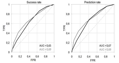
Figure 9 ROC plot and prediction rate curves comparison for the models. May 18th, 2015 and pre-event landslides included (black); only pre-event landslides included (grey)
Considering this scenario, the LR method was also applied using the entire landslide inventory (the multi-temporal and May 18th, 2015 MORLE-type event landslide inventories). In this case, the cross validation was performed by splitting the data into groups of 75% and 25% to train and validate each group. Figure 9 shows the ROC plot for the success and prediction rates compared to the model using only the multitemporal landslide inventory. Using the entire landslide inventory, the determined success rate was 0.65, and the prediction rate was 0.67. The results show that the final success and prediction rates do not improve, and the values slightly decrease.
According to these results, multi-temporal landslide inventories are more suitable for training and calibrating the landslide susceptibility assessment models, and MORLE-type events should be used carefully. To correctly determine the occurrence of landslides, it is necessary to include a past distribution of known landslides, including shallow and deep-seated landslides, related to different triggers, intense or prolonged rainfall events, or earthquakes59. Event landslide inventories should be used for temporal landslide validations; however, when using statistical methodologies, it is important to consider whether the landslide inventory used includes landslides with similar characteristics. In the case of tropical terrains, small shallow landslides are not preserved, and the landslide susceptibility assessment should only be considered for deep-seated landslides.
Finally, it is important to include all the causative factors, especially environmental variables, obtained directly from existing thematic maps or fieldwork. However, these variables are not available in regions with scarce data, such as tropical and mountainous terrains. This limitation indicates that the procedure proposed in this work is a preliminary approach to assess landslide susceptibility to guide the decision makers for land use planning. Detailed information and fieldwork are always required to determine the actual susceptibility conditions and reduce uncertainty.
Conclusions
Because areas affected by landslides are often remote and difficult to access, the landslide susceptibility assessment is often limited by the scarcity of reliable observations and available information. Hence, preliminary approaches are needed to identify landslide-prone areas. In this work, we consider a useful approach to assess landslide susceptibility in mountainous and tropical scarce-data regions using remote sensing data. Data availability is challenging for many researchers, especially in developing countries where many catchments remain remote and difficult to access. Google Earth satellite images and morphometric attributes derived from a DEM are increasingly available and used in landslide susceptibility assessments.
The Colombian Andes is a tropical and complex terrain that is periodically affected by landslides triggered by rainfall; however, large areas within this region lack essential data for landslide susceptibility and hazard analyses. The results of the Liboriana catchment, where on May 18th, 2015 104 people died, indicate that based on freely available DEM data and Google Earth satellite imagery, it is possible to obtain a landslide inventory and determine prediction factors to build an adequate landslide susceptibility model. Several strategies, such as the area under the ROC curve, the confusion matrix, the distance to the prefect classification, and the degree of fit, were implemented to validate the fit of the model and the prediction capability. In addition, the results showed that a large number of causative factors do not necessarily produce a better landslide susceptibility assessment.
Another important outcome is related to the completeness of the landslide inventory map using only remote sensing tools in tropical environments. Morphometric features of landslides are lost due to erosion or vegetation cover. Consequently, ancient shallow landslides are not included in landslide inventories, which reduces the prediction capacity of the statistical models to shallow landslides triggered by rainfall. To correctly determine the occurrence of landslides related to different triggers, it is necessary to include a complete past distribution of landslides.

