Introduction

A photonic crystal (PHC) is a device composed by several materials with different dielectric properties arranged periodically. Due to their important properties of controlling the propagation of light through stratified media ¹, such devices have greatly attracted the attention of the scientific community since the works of B. Bykov in the 1970s ² and the theoretical and experimental works of Yablonovitch during the 1980s ³. PHC have a great potential in the development of new optoelectronic devices, including optical fibers, sensors, optical circuits, metallic-dielectric arrays, frequency filters, films with high and low transmittance, among others ⁴, ⁵.

In order to study electromagnetic propagation through stratified media, several authors use the plane-wave expansion method (PWM), which helps to determine the propagation eigenmodes ⁶, ⁷. The finite-difference time-domain method FDTD ⁸, on the other hand, focuses on the dynamical behavior of the wave propagation without making special assumptions on the studied system; this property, in turn, allows to analyze several systems and so compare the transmission efficiency among complex optical structures.

Nonetheless, other authors ⁹ have considered the implementation of a matrix theory and use its mathematical properties to define operators that can determine the transmission and reflection (absorption, in some instances) amplitudes. Such formalism has been consolidated in the TMM ¹⁰, ¹¹, so providing an alternative method to study wave propagation ¹², ¹³ and encompassing the mathematical and numerical simplicity associated with a matrix theory. Additionally, this method allows us to study how the initial frequency of the wave influences its behavior in the media; numerically, the complexity of the calculations only varies logarithmically with the size of the system ¹⁴.

This document analyzes the dynamical behavior of the propagation of the electromagnetic radiation in stratified structures by means of the TMM ¹⁵. Although a general analysis includes multilayer systems with dielectric, conductor or semiconductor materials (or a combination of them), we focus on dielectric materials. We study how some variables, such as the width of the layers, the number of layers in the periodic array and how they are organized in the system, and the dielectric constants associated with the materials, influence the propagation of electromagnetic radiation in PHC's. Those are the variables usually studied by most authors and that can be controlled by the TMM ¹⁶. We briefly discuss how some of the systems that are analyzed can be used in current technology and compare some of our results with the ones of other authors.

Plane wave propagation through an interface by means of the TMM

We will start explaining the formalism that describes how the propagation of an incident wave is influenced when it passes through an interface. Figure 1 graphically describes this system and shows the notation that will be used. The initial and final media are dielectric semi-infinite media. Important results obtained by the academic community in this area include the study of semiconductor structures, such as porous silicon ¹⁷, Raman spectroscopy ¹⁸, and the analysis of morphological parameters of surfaces in multilayer systems ¹⁷. We will now present how the transmission and reflection coefficients in the TMM are obtained.

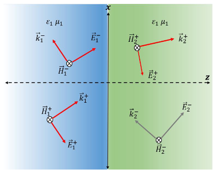
Figure 1. Graphical description of the propagation of an electromagnetic wave through an interface. The dielectric media are characterized by the permittivity and permeability constants ε1 and ε2, and μ1 and μ2, respectively. The subscripts 1 and 2 refer to the first and second media; E and H denote the electric and magnetic fields, k denotes the wave vector. 

The key point is to apply the continuity conditions for the longitudinal ("||") and tangential ("⊥") components of the electromagnetic fields respect to the interface ¹⁹. Let us thus consider an electromagnetic wave represented by the field \(\vec{E}_{r,t} = \vec{E}_{0}e^{i[k\cdot r - \omega t]}\) . For simplicity, the electric fields will be considered to be perpendicular respect to the interface, so \(\vec{E} = \vec{E}_{\perp}\) . Notice that Faraday's law implies that \(\vec{k} \times \vec{E} = \frac{\mu \omega}{c} \vec{H}\) and so the magnetic fields can be determined in terms of the electric ones. Hence, we can deduce the following relations

According to Figure 1, and using “+” to denote the fields propagating from left to right and “−” the fields propagating from right to left, the continuity conditions at the interface imply that

which can be represented in matrix form as

The column vectors at the left and right side of previous equation represent the amplitudes of the incoming and outgoing fields at each side of the interface: medium 1 and 2, respectively. Equation (5) can, in turn, be reorganized in terms of the transfer matrix \(M_{1 \rightarrow 2}\) , which can be expressed as

The transfer matrix \(M_{1 \rightarrow 2}\) stores the physical information of the media and the geometry associated with the propagation of the incident wave \((k_{i \perp} = \frac{\omega n_{i}}{c})\) . For the particular case of two semi-infinite media it coincides with the interface matrix between media 1 and 2, where \(\left( \begin{array}{c}E_{2}^{+} \\ E_{2}^{-} \end{array} \right) = M_{1 \rightarrow 2} \cdot \left( \begin{array}{c}E_{1}^{+} \\ E_{1}^{-} \end{array} \right)\) and the matrix elements of \(M_{1 \rightarrow 2}\) are \(M_{1 \rightarrow 2} = \left( \begin{array}{cc}(M_{1 \rightarrow 2})_{11} & (M_{1 \rightarrow 2})_{12} \\ (M_{1 \rightarrow 2})_{21} & (M_{1 \rightarrow 2})_{22} \end{array} \right)\) .

When the electromagnetic radiation comes exclusively from the left to the interface, we have \(E_{2}^{- } = 0\) . The transmission and reflection coefficients can thus be found using the linear system previously described; their respective probabilities are given by

where equations (7) and (8) are usually called the Fresnel coefficients ¹⁹ and can be used to write the interface matrix as

and can also be related to the matrix elements of the form

The transmittance and reflectance functions are finally defined as

Notice that the transmittance and reflectance function described in equation (11) depends on initial variables such as the frequency and normal angle of the incident wave. The dependence on the physical properties of the media, including their permittivities and permeabilities, is also clear by also noticing the dispersion relation in terms of the refractive index \(n_i\) as \(k_{i\perp} = \frac{\omega n_i \cos \theta_i}{c}\) .

Plane-wave propagation through an intermediate barrier

The following step is studying a system where the two semi-infinite media of previous section are separated by an intermediate barrier; this is graphically represented in Figure 3. This is an expansion of previous system, which, in turn, can be generalized when an arbitrary number of barriers is introduced. We now have three

Figure 2. Variable relation in the transfer matrix. 

media labeled by the indices \(\{1,2,3\}\) from left to right. Notice that we now have two interfaces, given by \((1 \rightarrow 2)\) and \((2 \rightarrow 3)\) . This configuration is usually called a rectangular barrier and has been studied in ²⁰ - ²², where the authors also mention some of its applications ¹².

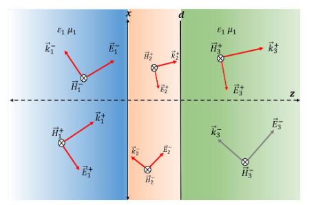
Figure 3. Graphical description of the wave propagation through a barrier of thickness a, whose dielectric are given by ε2, μ2. The orientation of the incoming and outgoing fields in the three media are also shown. 

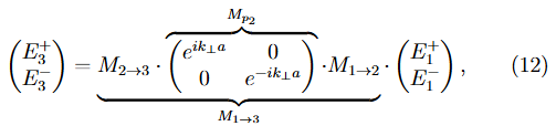
In the system, as represented in Figure 3, we once again assume that the incoming radiation comes from the left exclusively and advances in ascending numerical order (from 1, to 2, to 3). The new transfer matrix is thus the combination of two propagation matrices (from 1 to 2, \(M_{1 \rightarrow 2}\) and from 2 to 3, \(M_{2 \rightarrow 3}\) ) and a propagation matrix \(M_{p_{2}}\) (the subscript “2” refers to the second medium where the wave propagates) describing the propagation along the barrier. Therefore

or

The propagation matrix \(M_{p_2}\) considers multiple internal reflections within the homogeneous barrier (second medium) by means of plane waves of the form \(\vec{E}_2 = \left(E_2^+ e^{ik_{2\perp}z} + E_2^- e^{- ik_{2\perp}z}\right)e^{- i\omega t}\hat{y}\) . Using the results stated in equations (10) and (11), the new transmittance and reflectance functions can be defined as

If we consider a wave phase as \(\phi_2 = k_{2\perp}a\) , with \(k_{2\perp} = \frac{2\pi}{\lambda} n_2\cos \theta_2\) for the propagation matrix \(M_{p_2}\) within the second medium, it is possible to determine how the period of \(\phi_2\) will be \(\pi\) according to the angle of the incident wave within the range \(-\pi/2 \leq \theta \leq \pi/2\) . Therefore, by considering monochromatic incident light, constant thickness and refractive indices, it is possible to define the average transmission range within the barrier according to the condition

When last condition is satisfied, the wave oscillates within the barrier and generates interference. Otherwise, the system generates no interference and the transmittance function will show an approximate constant value. We can thus establish a condition for the maximum thickness necessary to obtain multiple reflections within the barrier, it is:

For instance, for light in the middle of the optical spectrum, with a wavelength of \(\lambda = 580\) nm, within the usual optical visible range of \(\Delta \lambda = 400\) nm, starting from air and passing through a medium with a refractive index of \(n_2 = 1.50\) under the condition of normal incidence, the maximum thickness satisfies the condition \(d_{max} < 0.280\) μm. This explains why, for the appropriate functioning of some optical devices, the thickness used in the fabrication of thin films must lie in the range of the wavelength of the incident light.

Simulation of transmittance spectra for optoelectronic systems

We can apply the previously explained results in order to model the transmittance function when a dielectric barrier of thickness \(a\) and refractive index \(n_2\) is introduced in a homogeneous medium such that \(\mu_1 = \mu_2 = \mu_3 = 1\) ; radiation propagates normally so \(k_{1\perp} = k_{3\perp}\) . According to equation (14), the transmittance function can be written analytically as

However, we can express previous function explicitly in terms of some of the parameters that describe the physical properties of the materials, so that

It is important to mention that the transmittance has a maximum value as the phase \(\phi = \frac{\omega n_2}{c} a = 0\) , or, in other words, as \(\frac{\omega n_2 a}{c} = m\pi\) , with \(m \in \mathbb{Z}\) . This maximum value will manifest periodically, so defining a period in the frequency domain where this is accomplished; this value is

Previous studies ²³ have determined that a wavelength of \(\lambda = 580\) nm passing through a glass barrier ( \(n_2 = 1.50\) , the initial and final media are air) shows a condition of maximum thickness given by \(d_{max} < 0.280\) μm under normal incidence. A value of \(n_2 = 1.5\) was used because it is the typical refractive index of glass, a common dielectric. Figure 4 shows the behavior of the transmittance function (and its associated reflectance) for a dielectric barrier immersed in vacuum and in presence of radiation in the optical range (from 400 nm to 700 nm), according to the thin layer condition expressed in ¹⁶ for a layer thickness of \(a = 270\) nm with normal incidence. Although the authors in ¹⁶ used a different refractive index than that used in ²³, interesting facts can be observed from the former data. Under these conditions, we can also observe the existence of regions where the minimum and maximum transmission and reflection alternate. This effect is caused by the configuration of physical parameters for the barrier, as anticipated in equations (16) and (19). The set of results obtained for such systems using the TMM can be extended to the study of some applications in daily life like coverings for photovoltaic cells (by means of multilayer systems), waveguides, and sensors. The characterization of optical materials can also be implemented via the Swanepoel method ²⁴, ²⁵, where the results obtained for the transmittance and reflectance are used to obtain information about energy gaps, dielectric function, and average thickness of the barrier, which are necessary variables to model optoelectronic devices.

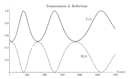
Figure 4. Transmittance (continuous line) and reflectance (dashed line) for a dielectric barrier of thickness 270 nm and refractive index n2 = 2.4 immersed in vacuum (n1 = n3 = 1.0). The graph was obtained by the authors using the formalism explained above. 

Nowadays, the design of covering layers in optoelectronic systems demands models suggesting characteristics such as small reflectance (high transmittance) ²⁶, a system that satisfies this condition is usually called an anti-reflective (AR) film. For instance, increasing the efficiency in photovoltaic systems depends on how we take advantage of the high-energy photons within the ultraviolet spectrum; it has been observed how coverings with high transmittance increase the efficiency of such systems between 2% and 17% ²⁷.

An additional barrier can be added to the system, similarly to the analysis presented in equation (12); we now must take into account three interface matrices and two propagation ones. This will allow us to study a system composed by a high transmittance film deposited on glass substrate. The main objective behind this idea is maximizing the transmittance function so that \(|T(n_{air}, n_{film}, n_{glass}, \omega , \lambda) - 1| < \epsilon\) , where \(\epsilon\) is a small enough number, so obtaining AR properties. For a thin layer deposited on a common glass substrate, the parameters associated with the materials must maximize the transmittance function ¹⁷; in order to accomplish this, the values shown in Table 1 will be assumed, see ²⁸ - ³⁰ for more details.

Table 1. Physical parameters used to model a high transmission dielectric film deposited in a substrate. 

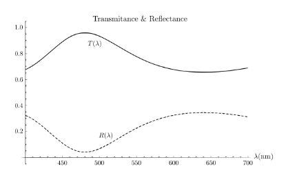
Once the system is simulated using the parameters shown in Table 1, and satisfying the condition previously mentioned, the results obtained for the transmittance and reflectance are shown in Figure 5. It is important to mention how the transmittance slightly exceeds the value 0.95 (continuous line) for an approximate value of \(\lambda = 480\) nm. In other words, the transmittance is maximized for wavelengths close enough to such value, which lie in the blue regime of the optical spectrum. Nonetheless, Figure 5 also shows how the transmittance significantly decreases far enough from such wavelength; this decrease goes down up to an approximate value of 0.7 in average.

Figure 5. Transmittance (continuous line) and reflectance (dashed line) for an anti-reflective film with a thickness of 200 nm and refractive index n = 1.23 deposited in an ordinary glass substrate with n_glass = 1.50 introduced in vacuum. 

Validation of the TMM for an AR multilayer

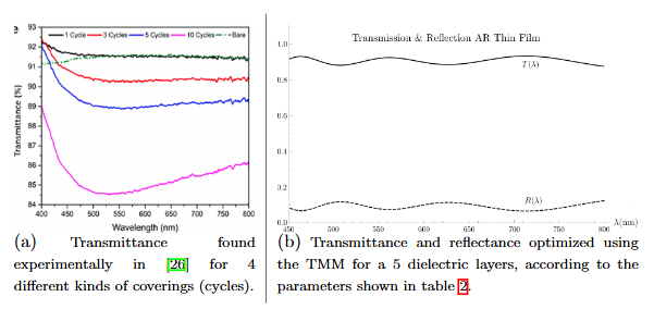
Aiming to confirm the accuracy of the TMM just proposed, we now pretend to extend the model to include 5 different layers. The objective is to test if the regions where the maximum transmittance is obtained can be extended to include a wider range of wavelengths that induce such condition. The finite difference method in the time domain FDTD has initially been used in ²⁶ to accomplish this. A graphical description is shown in Figure 6(a), comparing with Figure 6(b), which provides a graphical description of the approach using the TMM. Table 2 summarizes the optimal values found in ²⁶ using the FDTD method; the 5-layer-model implemented using the TMM will assume the same values.

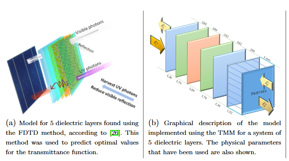
Figure 6. Graphical comparison between the FDTD method and the TMM for a dielectric multilayer system that maximizes transmittance. 

Table 2. Values that have been used for the refractive indices and thicknesses in the system of five layers that has been analyzed, according to ²⁶, where the model FDTD was implemented. 

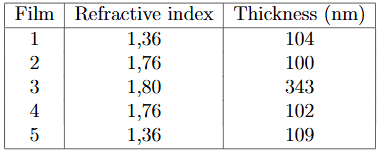
Figure 7 shows the spectra for maximum transmittance according to the mentioned parameters. While the figure in the left shows the experimental results found in ²⁶, the one in the right shows our results obtained using the TMM. Nonetheless, Figure 7(a) shows several spectra, each one corresponding to the number of cycles used in the deposition of thin films of (YVO4:Eu) and (HSNPs), as proposed in ²⁶.

The transmittance found using the TMM and shown in Figure 7(b) is similar to that found (experimentally) in Figure 7(a) for 1 cycle (black line). When the system is replaced by a single layer of ordinary glass, an approximate constant transmittance of about 0.94 is found, according to ³¹ (green line in Figure 7(a)); this value determines a maximum limit that should not be overcome in a system that includes additional layers. Comparing the results previously shown in Figure 5 with those that have just been presented, it is important to emphasize how the transmittance has increased, in the optical spectrum, in the multilayer system. The inclusion of additional layers in the substrate decreases the total reflection due to the internal reflections taking place in the different dielectric layers.

Figure 7. Comparison between experimental results and the ones obtained by the TMM for a multilayer system maximizing transmittance. 

PHCs wave guides

The next step associated with the analysis of the transmittance and reflectance in stratified media with dielectric media that are organized periodically is including the so called unidimensional photonic crystals PHCs ³², ³³. The PHCs are created by superposing homogeneous thin films (as defined in equation (16)) with well-known refractive indices. Such materials can have dielectric, conducting, or semiconducting properties ¹². First, an unitary cell is composed by \(n\) layers, dielectric in this case. Afterwards, \(N\) unitary cells are periodically superposed to create a large enough array. This final device exhibits useful properties, such as the appearance of very well-defined transmission forbidden/allowed energy bands ³⁴ and a minimum interaction between radiation and the medium, which can be explained though a null (or negligible) absorption in the frequency domain of interest. The appearance of transmission bands also emulates the behavior of semiconductors (respect to the electric charge transport) for certain potential values, called activation threshold ². That is why PHCs currently arise as one of the best candidates in the evolution of information transport; additional advantages include larger bandwidths for information transport, the possibility to modulate operational frequencies, low fabrication costs, and the possibility of creating devices that can operate at very low length scales ³⁵ - ³⁷.

The mathematical modeling of PHCs using the TMM is a generalization of the method used to analyze a barrier immersed in a homogeneous medium, which was explained before. Now, we build a unitary cell composed by \(n\) layers (see Figure 8 for a graphical representation, where a barrier is composed by two kinds of layers). If the barriers appear in the PHC with a periodicity \(\wedge\) , the refractive indices satisfy the periodic condition \(n_{z} = n_{z + \wedge}\) . Excluding the medium in which the PHC is immersed, the behavior of each unitary cell, with \(n\) barriers, and located at position \(m\) , is represented by the matrix

where, in terms of the perpendicular wave vector en medium \(j\) with thickness \(d_j\) ,

is a propagation matrix that account all the possible reflection within each particular barrier and \((M_{n\rightarrow n + 1})_{m} = (M_{n\rightarrow 1})_{m}\) when \(1 \leq m \leq N - 1\) , while \((M_{n\rightarrow n + 1})_{m = N} = M_{n\rightarrow N + 1}\) when \(m = N\) . Notice that, according to the notation that has been used and the periodic conditions, we have the restrictions \(U_{1} = U_{2} = \dots = U_{N - 1}\) ; \(U_{N}\) differs, as it takes into account the interaction of the PHC with the medium where it is immersed. Here we have also used the index " \(N + 1\) " to refer to the rightmost part of the system, which corresponds to the medium where the PHC is immersed (right limit); the index " \(0\) " will also refer to its counterpart (left limit).

Following this notation, the total matrix, the transfer matrix, can be written as

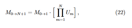
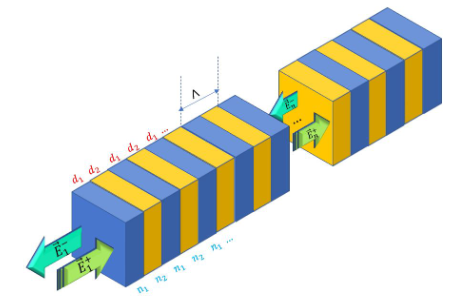
Figure 8. Graphical representation of a unitary cell composed by two different materials (n = 2) with thicknesses d1 and d2 respectively. There is a total of N unitary cells. 

so that the initial and final fields that propagate through the medium where the PHC is immersed are related by the equation

The transmission and reflection functions of the entire system are just an adaptation to equations (10) and (14), so

Notice that last relations do not necessarily assume that the medium from which the wave comes (left limit) and where it finishes (right limit) are the same. When they are, previous relation are greatly simplified.

Previous results can also be studied using the Bloch formalism, which focuses on the behavior of a single unitary cell and can also predict the appearance of forbidden/allowed bands. In this case, the electric field (magnitude, the field point in the \(y\) -direction, in our case) satisfies the relation

where \(\Lambda\) represents the spatial periodicity.

Therefore, for a wave that propagates within the \(j\) th layer, the fields satisfy the relations eigenvalue relation

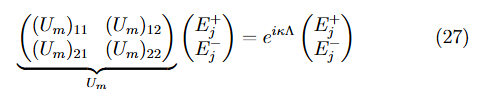
with solutions such that

taking into account that \(\det|U_{m}| = 1\) .

For a particular case, where we have a unitary cell composed by two layers (labeled by indices "1" and "2"), the real part of previous expression satisfies the condition ( \(\Lambda = d_{1} + d_{2}\) )

so the Bloch number finally takes the form

Equation (30) determines the conditions under which the Bloch wave propagates across the medium. When \(\frac{1}{2}\big((U_{m})_{11} + (U_{m})_{22}\big) > 1\) , the eigenvalues are real, thus providing the regimes where a wave does propagate; otherwise, when the eigenvalues are imaginary, the amplitude of the wave rapidly decreases and so a set of forbidden bands arises.

The behavior of the Bloch wave vector and the transmittance for a system with an unitary cell composed by two layers is shown in Figures 9 and 10. The refractive indices are \(n_1 = \frac{n_2}{4}\) , the thicknesses are equal, \(d_1 = d_2 = \frac{\pi}{2}\) and we used \(N = 5\) unitary cells. The PHC is immersed in air and the frequencies of the incident wave are considered within the visible spectrum. We can also observe, from Figure 9, how the Bloch vector is bounded \((0 < \kappa < \pi)\) for allowed frequencies out of which the band behavior arises. This band behavior defines regions of total transmittance or reflectance.

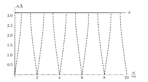
Figure 9. Behavior of the Bloch wave vector for energetic configurations allowed and forbidden for a unitary cell with two layers such that n1 = 1.5, n2 = 6.0 and d1 + d2 = Λ. We used a normalized value for κ in which Λ = 1. 

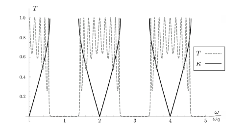
Figure 10. Behavior of the Bloch wave vector for energetic configurations allowed and forbidden for a unitary cell with two layers such that n1 = 1.5, n2 = 6.0 and d1 + d2 = Λ. We used N = 5. We used a normalized value for κ in which Λ = 1. 

On the other hand, Figure 11 describes the same behavior than that shown in Figure 10 but taking into account \(N = 10\) unitary cells. We can now appreciate a large number of resonances (compared to the last one) in the transmission band; however, their values and positions in the frequency domain do not change (the resonances are enveloped by the same curve).

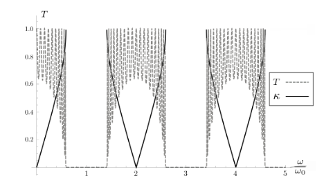
Figure 11. Behavior of the Bloch wave vector for energetic configurations allowed and forbidden for a unitary cell with two layers such that n1 = 1.5, n2 = 6.0 and d1 + d2 = Λ. We used N = 10. We used a normalized value for κ in which Λ = 1. 

Finally, Figure 12 shows the transmittance of a Bloch wave for a system with a unitary cells composed by two materials with \(n_1 = \frac{3}{5} n_2\) . The thicknesses are also equal \((d_1 = d_2)\) and \(N = 100\) . We can appreciate how the widths of the band gaps decreases as the difference between the refractive indices also decreases (the media behave similarly).

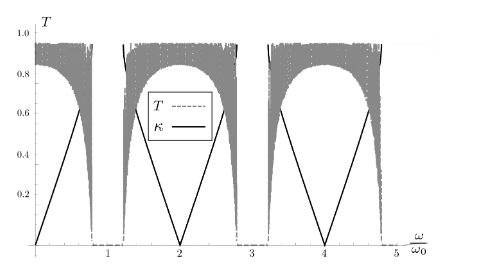
Figure 12. Behavior of the Bloch wave vector for energetic configurations allowed and forbidden for a unitary cell with two layers such that n1 = 1.5, n2 = 3.5 and d1 + d2 = Λ. We used N = 100. We used a normalized value for κ in which Λ = 1. 

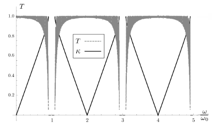
Figure 13. Behavior of the Bloch wave vector for energetic configurations allowed and forbidden for a unitary cell with two layers such that n1 = 1.5, n2 = 2.5 and d1 + d2 = Λ. We used N = 100. We used a normalized value for κ in which Λ = 1. 

From a theoretical perspective, mathematical modeling using the transfer matrix method provides a powerful tool to understand the interaction of light with periodic stratified structures. This approach enables us to predict and analyze phenomena such as transmission and reflection bands, as well as resonances that arise in these systems. From a practical standpoint, PHCs offer a range of technological advantages, such as the ability to control light transmission in specific frequency ranges, making them promising candidates for applications in optical devices, communications, and sensors.

Conclusions

The TMM offers the possibility of studying the characterization of optical materials with different construction properties, materials, and purposes. The mathematical simplicity of this method is evident; once the formalism for a single barrier is understood, and analytical expression are found, the generalization for several layers and unitary cells is straightforward. Although numerical methods, including the one studied in this document, give great advantages to approach the study of real systems, there exist other analytical models that allow to include the effects of different parameters, each one implemented according to experimental needs and that could provide a better approximation level ¹⁴. Nonetheless, the simplicity behind the formalism, is an important first step to anticipate which kinds of materials and configurations may generate devices with the properties that are needed in current technology.

The comparison between the plane-wave expansion method and the TMM highlights advantages and specific limitations associated with each formalism in the analysis of periodic structures and wave propagation. The former method turns out to be more exact to compute dispersion bands in infinite periodical systems; however, the more complex the structure to be analyzed, the more computational cost is demanded. On the other hand, the TMM is more efficient to study finite multilayer systems, a limitation arises as errors accumulate in multilayer systems, though. Selecting the most appropriate method depend on the characteristics of the system; a combination between both methods can be sometimes implemented to take advantages of such approaches ³⁸, ³⁹.

Independently of the theoretical method used, PHC offer a great alternative to create new materials that enable to transmit information more efficiently. Some of the advantages of these systems include the modeling of the wave guide, as well as allowing the introduction of new applications in optoelectronics.

For a set of stratified media, the transmission band structure and the forbidden gap, associated with how a PHC reacts to the propagation of light was numerically determined. The behavior of these bands was analyzed, showing how the dielectric properties of the media, the geometry of the PHCs, as well as the number of unitary cells taken into account affect them. This shows the possibility of adjusting such parameters to construct a particular device, with the set of properties needed for a particular task.