English (pdf)
 Article in xml format
 Article references
 Send this article by e-mail
 Cited by SciELO
  Cited by Google
  Similars in
SciELO
Similars in
SciELO  Similars in Google
 Permalink
1 Introduction
The Burr distribution was formally presented in 1942, as part of a family of useful distributions for fitting data [1]. Among the initial list of twelve parametric functions given as solution examples of the differential equation being analysed, the last one, usually called the Burr XII or simply the Burr distribution, is the most popular. Part of the advantages of the three-parameter Burr XII distribution, sometimes also called Singh-Maddala distribution, arises from the flexibility that it provides, including that some other practical and well know distributions such as the Pareto, Weibull, Log-logistic, and Paralogistic can be obtained as a special case of the Burr XII model.
There are different applications of the Burr distribution to model data in a wide range of areas. In actuarial science, it is used to model the size of insurance claims, especially for heavy-tailed distributions [2,3, 4, 5]. In reliability analysis, this distribution is used to model failure rates of components [6, 7]. In survival analysis, it is used to model lifetime variables [8, 9]. In economics, it is used to model income distribution [10]. It has also been used in finance [11] and engineering [12,13].
Several authors have used ML to estimate the Burr Type XII distribution parameters under different scenarios of incomplete censored data. Among those, we can mention type II censored data [14], progressively censored data [14], multiple-censored and singly-censored data (Type I censoring or Type II censoring) [15], random censored data [16] and middle-censored data [17]. Similarly to data modifications by censoring, but to a lesser extent, other authors have analyzed the Burr XII distribution under truncated data conditions [18, 19]. Some authors have also studied parameter estimation under data of various lifetime distributions with some censoring and truncation simultaneously [20, 21, 22,23].
In addition to estimation developments under data modifications, research has also focused on extended models of the three-parameter Burr XII distribution, including its properties and related applications. Some of these extensions can be obtained by adding parameters; included are a four-parameter model called the Weibull Burr XII distribution [24], a five-parameter distribution called the Kumaraswamy Burr XII distribution [25], a six-parameter generalized Burr XII distribution [26] and even a seven-parameter Burr distribution [27]. Additional extended models can also be obtained using other mathematical techniques [28,29, 30,31] or definitions of the density function [32].
This paper focuses on estimating the three-parameter Burr XII distribution parameters via MLE when data are simultaneously left-truncated and right-censored. Section 2 describes some properties of the Burr distribution and introduces the definition of left-truncated and right-censored data. Section 3 presents the ML function for the Burr distribution with truncated and censored data. In Section 4, the MLE equations are solved, and the observed Fisher information matrix is obtained. Section 5 describes how to estimate confidence intervals for the parameters. A simulation study is implemented in section 6. Applications to real data are presented in Section 7. The paper ends with a short discussion and suggestions for further research in Section 8.
2 Background
This section describes the Burr XII distribution and its properties and reviews the definitions of truncated and censored data.
2.1 Burr XII Distribution
The parametrization for the Burr XII distribution follows [3] and corresponds to the way it is usually presented in the actuarial literature, where it has gained significant attention in the last two decades. A random variable X is said to have a three-parameter 0 = (a, y, 6) Burr XII distribution, or simply a Burr XII distribution, if its density and distribution functions are given by
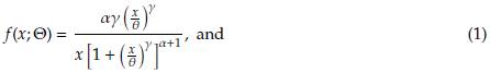
where α and γ are shape parameters and θ is a scale parameter. In order to illustrate its flexibility, some forms of the density and distribution functions are shown in Figure 1.
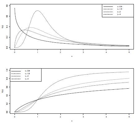
Figure 1: Densities and distributions functions of Burr XII ditributions with parameters α = 0.5, θ = 1 and y = (0.9,1.5,2,4), respectively.
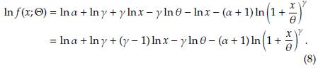
Given a random sample, x 1 , . . . , x n , of a Burr XII distribution, the log-likelihood function can be written as
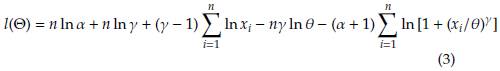
Taking the derivative of l(Θ) in (3) with respect to the parameters α, θ and γ and setting them equal to zero we have
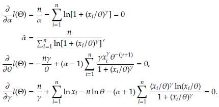
There is not an explicit solution for θ and y above, and therefore some numerical method such as Newton-Raphson needs to be used.
2.2 Left Truncated and Right Censored Data
In practice situations it is usual that complete information is not available and the researcher is only disposed incomplete data. In survival and reliability studies the interest is on the non-negative random variable representing the time until the occurrence of an event, usually the time of death or failure of a component. A common example of incomplete information is when the failure time data includes information from individuals who did not fail in the observation period or were only observed up until certain point of time; this information is said to be right censored and it is incomplete since the survival time goes beyond the observed point, but the exact time of failure is not known.
A second source for incomplete information arises when only individuals who experience some event are observed; that is, individuals are followed in the study only if they fulfill a required condition which screens them in order to be included in the analysis. This produces a biased sample, and those who are observed are said to be left truncated. It is usual to have left truncated data when individuals have a delayed entry or when they do not survive until the beginning of the observation period.
In insurance, the main variables of interest are the number of claims and the size or value of those claims. Left truncation occurs if the insurer pays only when the value of the claim is more than an agreed amount d, called the deductible. Right censoring arises with a policy limit u, where even if the loss exceeds the pre-established amount u, benefits are paid only up to u.
In survival analysis, as well as in insurance, it is very common to have data that is left truncated and right censored (LTRC) simultaneously. An observation is right censored (or censored from above) at u if when it is at or above u it is recorded as being equal to u, but when it is below u it is recorded at its observed value. On the other hand, an observation is left truncated (or truncated from below) at d if when it is at or below d it is not recorded, but when it is above d it is recorded at its observed value [3].
3 Log-Likelihood Function for the Burr XII Distribution with LTRC Data
It is well known that under complete individual data, the contribution to the likelihood function from an individual with exact observed lifetime of xi is the corresponding density function, notated by f (x
i
; Θ) where Θ = (θ1, θ 2,..., θ
n
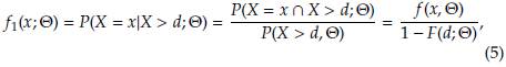
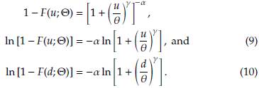
) is the parameter vector of the distribution. However, when dealing with incomplete data, the construction of the likelihood function needs to be carefully considered in order to account properly for the information given in each sampled observation. If the observation comes from a population with left truncation at d, then it should be noted that it was observed given that its value exceeded d, and therefore the (conditional) contribution to the likelihood function from a left truncated observation is

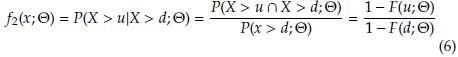
For a right censored observation at u, all we know is that its value exceeded u, thus the contribution to the likelihood function from a right censored observation is simply (1 - F(u; Θ)), that corresponds to the probability of exceeding u. Consider a sample of n + m data left truncated at d, where m of them are also right censored at u. The likelihood function, for a data set with these characteristics, is given by
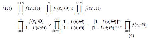
with
and
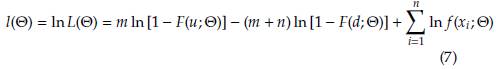
Taking logarithms in (4) we obtain the log-likelihood function as follows
From (1)
From (2)
Replacing (8), (9) and (10) in (7) we obtain the log-likelihood function for the Burr XII distribution with censored and truncated data. This is given by
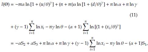
with
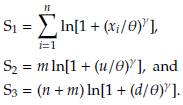
Notation S1 , S2, S3 is given in [15].
4 Parameter Estimation of the Burr XII Distribution with LTRC Data
Taking the derivative in Equation (11) with respect to a, and setting it equal to zero we have
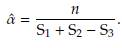
Defining
the likelihood equations for 6 and y are
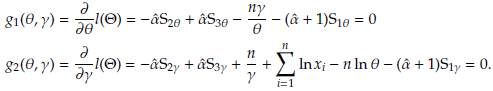
The equations for θ and γ can be written in matrix notation as
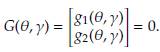
The MLE of θ and y are the values
 and
and
 that simultaneously solve this non-linear equation system. An option in this scenario is to use the iterative Newton-Raphson method [33]. According to this approach, the iteration (k + 1) to solve the system is
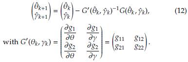
Equation (12) can be simplified as
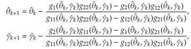
where
 0,
0,
 0, and
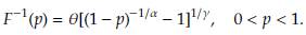
 0 are values for the starting points. A good choice of these is important to improve convergence. Generally the method of moments (MM) or percentile matching method (PM) are used to set the initial values. From a computational point of view, it is preferable the second option [3] since the MM also requires to solve a system of equations using numerical methods. The PM consist of replacing theoretical percentiles with empirical percentiles of the random sample. In the case of a Burr XII distribution the quantile function is defined as
For example, let us assume that
 1,
1,
 2 and
2 and
 3 are estimations of percentiles p
1
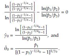
= 25th, p2 = 50th and p3 = 75th, respectively. It can be shown that
3 are estimations of percentiles p
1
= 25th, p2 = 50th and p3 = 75th, respectively. It can be shown that
 and
and
 are obtained by solving the following equations
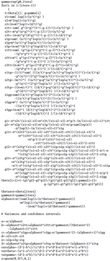
5 Covariance Matrix and Confidence Intervals
ML estimators are asymptotically normal estimators with variance and covariance given by the inverse of the Fisher information matrix l(Θ). When certain regularity conditions are met 7(Θ) can be approximated by the observed Fisher information matrix [34], notated 1(
 ) and given by
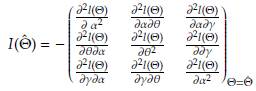
From Equations (5) and (6) it can be seen that for a fixed truncation point d and a censoring point u the contribution of LTRC to the log-likelihood function preserve the functional form of the log-likelihood function of a Burr XII distribution with complete data; therefore, the existence of the Fisher information matrix for LTRC data is guaranted. To verify the later we refer the reader to papers such as [35] and [36]. The approximate covariance matrix can be estimated as
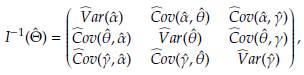
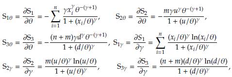
where
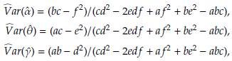
with (see appendix)
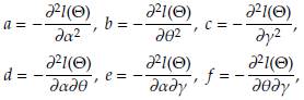
all of these evaluated at the estimated parameters
 and
and
 Based on asymptotic normality of ML estimators, confidence intervals of 100(1 - ρ)% for
 are defined as
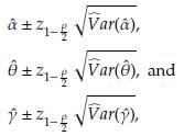
where
 is a quantile of a standard normal distribution.
6 Simulation Study
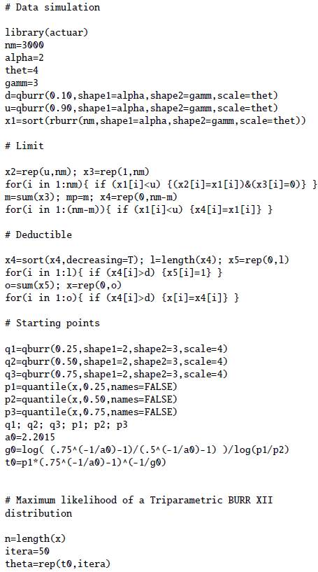
Initially, in Section 6.1, we graphically establish the goodness of fit of the proposed methodology. Subsequently, in Sections 6.2 and 6.3, a more intensive computational study is carried out to study empirically the convergence of the estimators. The R code used in the simulations is given in Section 9 and is also available at the web page https://sites.google.com/a/unal.edu.co/ramon-giraldo-webpage/r-code (see RCodeBurrXII.R).
6.1 Goodness of fit test for the Burr XII (α = 2, γ = 3,θ = 4) distribution
Using the R library actuar [37] 1000 data from a Burr XII distribution (α = 2, y = 3, θ = 4) are simulated (histogram in Figure 2). A large data set is used to have a good approximation to the population distribution. The data generated are posteriorly left truncated at d = 1.51 and right censored at u = 5.17 (dashed vertical lines in Figure 2) obtaining 796 observations in the interval (d, u]. Using these partition of the data and the iterative procedure described in Section 4, the MLE are obtained. The 25th, 50th, and 75th percentiles of the generated data are 2.29, 2.98, and 3.76, respectively. The starting points are calculated using these values and the PM method (see Section 4). These are
 0=2.20,
 0=3.71, and
 0=3.89, respectively. The final estimates are
=1.93, y=2.98, and
=3.93. The estimated density function (dashed curve in the interval [1.51, 5.17] in Figure 2) is very close to the reference density (continuous line in Figure 2) and consequently suggests that the approach implemented is satisfactory.
0=3.89, respectively. The final estimates are
=1.93, y=2.98, and
=3.93. The estimated density function (dashed curve in the interval [1.51, 5.17] in Figure 2) is very close to the reference density (continuous line in Figure 2) and consequently suggests that the approach implemented is satisfactory.
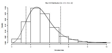
Figure 2: Histogram density estimation of 1000 simulated data from a Burr XII distribution with α = 2, γ = 3, and θ = 4. Data are left truncated and right censored at 1.51 and 5.17, respectively (vertical dashed lines), The black line corresponds to the Burr XII density, and the dashed curve (between 1.51 and 5.17) to the estimation of a Burr XII left truncated and right censored.
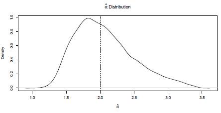
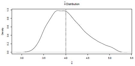
Figure 3: Kernel density estimation of the a distribution. Values obtained from 10000 size n = 1000 Monte Carlo simulations of X ~ Burr XII (α = 2, y = 3 and θ = 4). Dashed vertical line allows identify the parameter a. Burr XII Distribution (o= 2 g= 3 9 = 4)

6.2 Distribution of the estimators
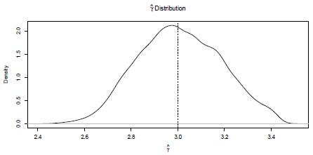
10000 simulations size n = 1000 of a Burr XII distribution (α = 2, γ = 3, θ = 4) were run. Each random sample simulated is trimmed at d=1.51 and u=5.17. At each iteration the Newton-Raphson algorithm is carried out (based on 100 iterations) and the parameters are estimated. If the starting points are not properly defined the method fails. Approximately 70% of the runs allow obtaining the estimates of the parameters. Kernel density estimations obtained for
 ,
,
 and
and  are shown in Figures 3, 4, and 5. These plots suggest that is reasonable assuming asymptotic normality for the distributions of
and
. The distribution of
are shown in Figures 3, 4, and 5. These plots suggest that is reasonable assuming asymptotic normality for the distributions of
and
. The distribution of
 is slightly biased. A large sample size n could be required in this case.
The means of the corresponding estimations (vertical dashed lines) are 1.98, 2.98, and 3.93. These values are very similar to the parameters. The curves in Figures 3 to 5, indicate that in general the methodology used presents a good performance.

6.3 Comparison of results varying n and θ
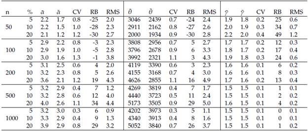
A computationally intensive simulation procedure was conducted. 10000 simulations size n = 50,100,200,500, and1000 of Burr XII distributions were generated. At each case following the methodology proposed were estimated the parameters (α, θ, γ). Three levels of censure and truncation (5%, 10%, 20%) are considered. Summary statistics (mean, median, coefficient of variation, relative bias, root mean square error) were calculated based on the estimations. As in Section 6.2 the final number of estimations depends on the convergence rate of the method which is around 70%. The results are shown in Tables 1 and 2. Various points can be highlighted from these Tables. In general, the greater the number of censored and truncated observations the greater the relative bias and the root mean square error. There are differences between means and medians which indicate the presence of some atypical estimated values. As expected, according with the root mean square errors (RMS), the more data for model fitting the better the estimations, i.e., the estimators are asymptotically unbiased.
7 Applications
We now consider two examples with real data. Although both data sets have been used to fit a Burr XII distribution, they are modified to adjust them to left truncation and right censoring conditions. An R [38] code is used to compute ML estimations with LTRC data. The code allows solving the adjusted ML equations (given in section 3) using the Newton-Raphson algorithm. The starting points are obtained from the PM with the 25th, 50th, and 75th percentiles. 95% confidence intervals for the parameters are obtained. Plots comparing empirical and fitted distributions are presented. A KS test, adjusted to incomplete data, is used to assess the goodness of fit.
7.1 Breast Cancer Data
The information corresponds to breast cancer survival data of 935 patients [39]. The study was carried out between 2009 and 2013. 705 people were still alive at the end of 2013 (data are censored at u = 1826). The frequency histogram is shown in Figure 6. A log transformation of frequencies is used to reduce the scale. We observe a high frequency on the right of the distribution which is due to the censored information. The data set is artificially trimmed in order to left truncate it by considering a truncation point at d = 30 days. Thus, a new data set is obtained by eliminating the 9 points that are below 30 from the adjusted set, resulting in 221 patients with exact observed times and 705 with censored information. Here we take into account censored and truncated data to estimate the parameters. 1000 Survival(days)
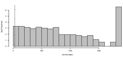
Figure 6: Frequency histogram of breast cancer survival data. A log transformation of frequencies is used to reduce the scale. High frequency at the end of the distribution is due to censored data. Data are left truncated at d = 30 (dashed line) and right censored at u = 1826 (last interval).
From available information, initial estimates (
 0 = 0.26,
 0 = 2.84, and
 0 = 201.51) of the parameters were obtained by using the PM. The final estimates after using the methodology proposed are
 = 0.08,
 = 1.57,
 = 182.96.
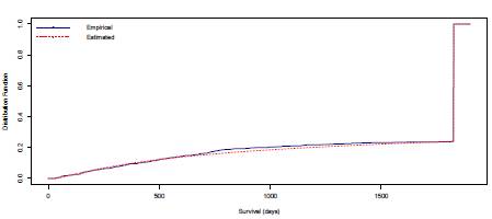
A comparison between the empirical and estimated distribution functions is shown in Figure 7. The estimated distribution is obtained from a simulation size 10000 of a Burr XII ( = 0.077,
 = 1.566,
= 182.96) model. We can observe graphically that the model fitted seems appropriate. The p-value of a KS goodness of fit test conducted to compare the distributions in Figure 7 is 0.83. According to this value there is not statistical evidence to reject the hypothesis that breast cancer survival data can be fitted with the Burr XII distribution estimated. 95% confidence intervals for α, γ, and 6 were obtained.
= 1.566,
= 182.96) model. We can observe graphically that the model fitted seems appropriate. The p-value of a KS goodness of fit test conducted to compare the distributions in Figure 7 is 0.83. According to this value there is not statistical evidence to reject the hypothesis that breast cancer survival data can be fitted with the Burr XII distribution estimated. 95% confidence intervals for α, γ, and 6 were obtained.
These are respectively [0.072, 0.079], [1.413, 1.719], and [140.301, 225.629].
7.2 Bladder Cancer Data
The data correspond to remission times from patients with bladder cancer as described in [40]. A subset of this data was used in [41] to fit a log-logistic distribution (a particular case of a Burr XII distribution). The frequency histogram is shown in Figure 8. This data set is truncated from below at d = 2 (dashed line in Figure 8) and censored from above at u = 30. The ML estimates for the parameters of the Burr XII model are a = 2.33, y = 1.23 and 6 = 12.50. A comparison between the empirical distribution function (generated from the data recorded) and the theoretical distribution function (obtained from 10000 simulated data of a Burr XII model (a, y, 6)) is presented in Figure 9. This graph validates from a descriptive point of view the methodology used.

Figure 8: Frequency histogram of bladder cancer remission times. Data are left truncated at d = 2 (dashed line) and right censored at u = 30 (last interval).
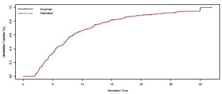
Figure 9: Distribution functions (empirical and estimated) for remission times (bladder cancer data)
Table 1: The parameters are α = 2, θ = 4, and γ = 3. n: sample size. %: Percentage of censure and truncation. For example 5% means 2.5% of censure and 2.5% of truncation.  and
and  are the means and medians of the estimations, respectively. CV: Coefficient of variation of the estimations. RB: Relative bias %. RMS: Root mean square error.
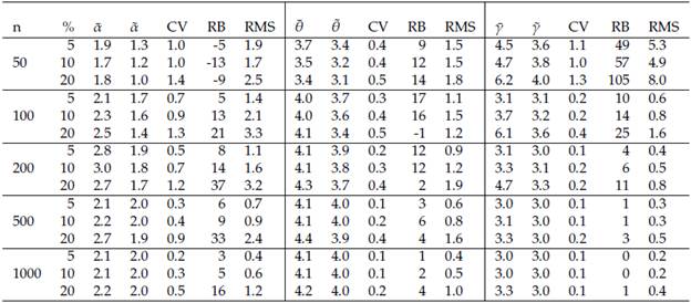
Table 2: The parameters are (a = 2, 6 = 4000, y = 3). n: sample size. %: Percentage of censure and truncation. For example % = 5% means 2.5% of censure and 2.5% of truncation. and are the means and medians of the estimations, respectively. CV: Coefficient of variation of the estimations. RB: Relative bias %. RMS: Root mean square error. For simplicity in the presentation RMS values corresponding to the estimation of 6 are divided by 1000 and rounded to one decimal.
A KS test was conducted to formally compare these cumulative distributions. The p-value obtained (0.997) corroborate the graphical results described. 95% confidence intervals for a, y, and 6 are respectively, [1.95, 2.72], [0.90, 1.57], [8.86, 16.15].
8 Conclusion
The Burr XII distribution is useful to model data in several areas, including applications in survival analysis, actuarial science, and reliability theory. Its flexibility and closed form, among other statistical properties, are some advantages when it is compared with other distributions. In many real situations it can be required to work with left truncated and right censored data. In this work we propose a methodology to estimate the parameters of the Burr XII distribution in this context. We use numerical methods to estimate the parameters by ML. We also give an approach to estimate the variances and covariances matrix and therefore to calculate confidence intervals. In order to illustrate the methodology, a simulation study and two real data analysis are carried out. In both scenarios, the results indicate that the methodology proposed has a good performance. This work can be extended to include other types of data modifications that also arise in practice; in addition it can be applied to other family of distributions where LTRC data are naturally found.