


 English (pdf)
 Article in xml format
 Article references
 Send this article by e-mail
 Cited by SciELO
  Cited by Google
  Similars in
SciELO
Similars in
SciELO  Similars in Google
 Permalink
1 Introduction
Several methods have been proposed in the statistical literature to test the equality of mean vectors for two p-variate normal populations. This problem, commonly referred to as the Behrens-Fisher problem, is defined by the following set of hypotheses:
For example, if we are comparing two species (1 and 2) of penguins according to flipper length and body mass, the vectors μ 1 and μ 2 contain the means of these two measurements for species 1 and 2, respectively.
The Hotelling test is one approach to tackle this problem, assuming equality of the two covariance matrices. However, this test has limitations when the variance and covariance matrices are unknown and unequal. To address these deficiencies, several alternative methods have been developed with the aim of obtaining hypothesis tests that yield more consistent and efficient results.
The earliest solutions to this problem were proposed by Bennett [2] and James [6]. Bennett's solution was based on the univariate solution presented by Scheffé [15], while James extended the univariate Welch series solution. Yao [19] proposed an extension of the Welch approximate degrees of freedom and conducted a simulation study comparing it with James' solution. Johansen [7] presented an invariant solution within the context of general linear models and obtained the exact null distribution of the statistic. Nel and Van Der Merwe [12] also obtained the exact null distribution of the statistic and proposed a non-invariant solution. Kim [10] introduced another extension of the Welch approximate degrees-of-freedom solution, utilizing the geometry of confidence ellipsoids for the mean vectors. Krishnamoorthy and Yu [11] proposed a new invariant test by modifying Nel's solution. Gamage et al. [4] proposed a procedure for testing the equality of mean vectors using generalized p-values, which are functions of sufficient statistics. Yanagihara and Yuan [18] suggested the F test, Bartlett correction test, and modified Bartlett correction test. Kawasaki and Seo [9] proposed an approximate solution to the problem by adjusting the degrees of freedom of the F distribution.
In the context of conducting Hotelling's T 2 test for multivariate data assuming equality of the covariance matrices, several R packages provide useful functions. The ICSNP package offers the HotellingsT2 function, the rrcov package includes the T2.test function, the Hotelling package, with its hotelling.test function, and the Compositional package offers the comp.test function (Hotelling and James). However, those packages do not provide functions to perform the tests proposed by James, [15], [19], [7], [12], [10], [11], [4], [18] and [9] when the covariance matrices are unequal.
This paper is organized as follows: Section 2 provides an overview of the statistical tests implemented in the stests R package which is a programming language and software environment specifically designed for statistical computing created by the R Core Team [13]. In Section 3, an introduction to the stests R package, which was created to implement these statistical tests, is presented. Sections 4 and 5 detail the design and results of a simulation study conducted to compare the statistical tests. Lastly, Section 6 contains conclusions and discussion.
2 The Behrens-Fisher problem
The univariate version of the Behrens-Fisher problem was proposed initially by Behrens [1] and then reformulated by Fisher [3]. The problem concerns comparing the means of two independent normal populations without assuming the variances are equal. The multivariate version of the Behrens-Fisher problem refers to a statistical hypothesis testing dilemma concerning the comparison of two population means when the variances of the populations are unequal. The interest can be summarized as follows:
Let x i1, x i2,..., x ini a random sample from a p-variate normal population N(μ i, Σ i) with i = 1,2. The Behrens-Fisher problem has the next set of hypotheses:
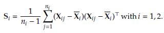
The tests proposed in the literature require specific inputs, namely the sample mean vectors and sample covariance matrices, to perform the necessary calculations. The expressions to obtain these inputs are as follows:
and the sample variance-covariance matrices
Next, the statistical tests implemented in the stests R package to study the hypothesis given in expression (2) are listed.
Hotelling test.
First order James' test (1954).
Yao's test (1965).
Johansen's test (1980).
NVM test (1986).
Modified NVM test (2004).
Gamage's test (2004).
Yanagihara and Yuan's test (2005).
Bartlett Correction test (2005).
Modified Bartlett Correction test (2005).
Second Order Procedure (S procedure) test (2015).
Bias Correction Procedure (BC Procedure) test (2015).
All of the tests listed above have expressions for the statistics and their distributions under the null hypothesis. However, due to the length and complexity of these expressions, it is recommended that readers refer to the vignette available in [5] for detailed information. The vignette provides comprehensive explanations, equations, and examples related to the statistics and their distribution, allowing readers to delve into the specifics of each test.
3 The stests package
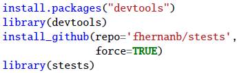
In this section, we introduce the stests R package, which has been developed to facilitate the implementation of multivariate statistical tests for the Behrens-Fisher problem. The package is currently available on the GitHub platform, allowing users to easily download and utilize it. To install and use the package, users can use the following code snippet:
The main function of the stests package is two_mean_vector_test(). This function has the next structure:
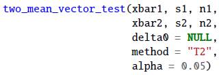
The arguments xbar1, s1, and n1 correspond to the sample mean vector, sample covariance matrix, and size of the sample 1. In the same way, xbar2, s2, and n2 are the information for the sample 2. The argument delta ∅ is a p-dimensional numeric vector to test H0: μ 1 - μ 2 = δ0, by default, δ0 = 0.
The method argument can be used to indicate the name of the hypothesis test, the current values are "T2" (default), "james" (James' first order test), "yao" (Yao's test), "johansen" (Johansen's test), "nvm" (Nel and Van der Merwe test), "mnvm" (modified Nel and Van der Merwe test), "gamage" (Gamage's test), "yy" (Yanagihara and Yuan test), "byy" (Bartlett Correction test), "mbyy" (modified Bartlett Correction test), "ksl" (Second Order Procedure), "ks2" (Bias Correction Procedure). Finally, the alpha argument is used only to obtain the critic value for the James test.
The two_mean_vector_test() function generates an object of class htest. For this type of class, we create the general S3 functions print() and plot(). In the examples below, we illustrate the utility of these functions.
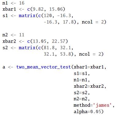
3.1 Example 1
Here we revisit example 3.7 from Seber [16] on page 116, using the James first-order test to explore the null hypothesis H0: μ 1 = μ 2, with a significance level of a = 0.05. We can use the function two_mean_vector_test() with the argumentmethod="james". The resulting output is stored in the object a.
We can write in the R console the object name a to obtain the next summary for the test.
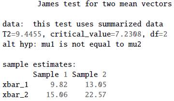
From the summary, we note that the critical value is 7.2308, and the test statistic 9.4455. For this reason there is evidence to reject H0: μ 1 = μ 2
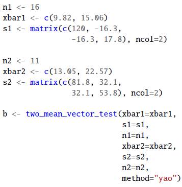
3.2 Example 2
In this second example we used the data from Yao [19] on page 141. The objective is to test H0: μ 1 = μ 2 versus H0: μ 1 ≠ μ 2 using the Yao test. We can use the function two_mean_vector_test() with the argument method="yao". The resulting output is stored in the object b.
We can write in the R console the object name b to obtain the next summary for the test.
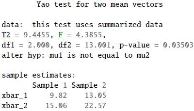
From the summary, we observe that the p-value is 0.03503, which is lower than the conventional significance level of 5%. Therefore, there is evidence to reject the null hypothesis H0: μ 1 = μ 2 .
4 Simulation study
A Monte Carlo simulation was conducted to evaluate the performance of the function developed for the Behrens-Fisher tests. In the simulation study we considered four factors:
• p: the dimension of the two normal populations, three cases were considered, p = 2, p = 3 and p = 5.
• n: the same sample size for both populations was equal (n1 = n2 = n) with values n = 10,20,..., 150.
• δ: distance between the components of centroids μ 1 and μ 2 . For p = 2, the values for δ were 0,10,20,..., 150. For p = 3, the values for δ were 0,10,20,..., 150. For p = 5, the values of δ were 0,0.5,1.0,1.5,..., 7.0,7.5.
• k: a scalar factor to relate the variances and covariances matrices, that is, Σ2 = k · Σ1. The values considered were k = 1,2,5, where k = 1 means that both variances and covariances matrices are equal.
The combination of the aforementioned factors produces 1440 scenarios. For each scenario, 1000 samples of size n were generated from both p-variate normal populations using the mvrnorm function of the MASS package of [17].
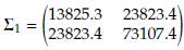
When p = 2, the baseline mean vector and variance-covariance matrix were taken from example 4.1 by Nel and Van Der Merwe [12], located on page 3729. The baseline mean vector for population 1 was held fixed at μ 1 = (204.4, 556.6) while μ 2 was obtained by adding δ to each component of μ 1. The baseline variance-covariance matrix Σ1 was
When p = 3, the baseline mean vector and variance-covariance matrix were taken from excersice 6.18 by Johnson and Wichern [8], located on page 344. The baseline mean vector for population 1 was held fixed at μ 1 = (113.4,88.3,40.7) while μ 2 was obtained by adding δ to each component of μ 1. The baseline variance-covariance matrix Σ1 was
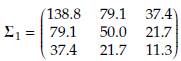
When p = 5, the baseline mean vector and variance-covariance matrix were taken from example 3.10.1 by Rencher and Christensen [14], located on page 79. The baseline mean vector for population 1 was held fixed at ft = (36.09, 25.55, 34.09, 27.27, 30.73) while μ 2 was obtained by adding δ to each component of ft. The baseline variance-covariance matrix Σ1 was
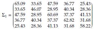
The variance-covariance matrix Σ2 was obtained as Σ2 = k · Σ1. If a valid variance-covariance matrix Σ is multiplied by a positive scaling factor k, the resulting matrix retains the property of being positive definite.
The performance of each test in the simulation study was measured by the rejection rate of the null hypothesis, which is the probability of rejecting the null hypothesis when it is actually true. It is also known as the Type I error rate or significance level. The rejection rate is typically denoted by the Greek letter α (alpha).
To calculate the rejection rate, you need to specify a critical value or a range of critical values based on the desired significance level. The critical value(s) define the boundary between the region where the null hypothesis is rejected and the region where it is not rejected. The rejection rate can be expressed as:
For the James test [6], we did not calculate the p-value because there is no distribution for the statistic, so the critic value was used to calculate the proportion of rejections of H 0. In the simulation study, the significance level was constant at α = 0.05.
5 Results
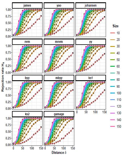
The rejection rates of the null hypothesis H0: μ 1 = μ 2 for scenarios with p = 2 are illustrated in Figures 1 to 3. When δ = 0 the null hypothesis is true, the rejection rates of H 0 are approximately 0.05. Furthermore, as the value of δ increases, indicating that the null hypothesis is false, the rejection rates progressively approach 1.00. Therefore the rejection rates of the null hypothesis increase as the discrepancy between the mean vectors μ 1 and μ 2 becomes larger.
Upon observing Figures 1 to 3, it is evident that as the scaling factor k increases, the rejection rate of the null hypothesis decreases. This suggests that a larger scaling factor leads to a more conservative test, resulting in a lower probability of rejecting the null hypothesis.
Furthermore, it can be observed that as the sample size n increases, the rejection rate also increases. This implies that with larger sample sizes, the statistical test becomes more powerful in detecting differences between the mean vectors, leading to a higher probability of rejecting the null hypothesis when it is indeed false.
Figures 4 to 6 depict the trend of the rejection rates of the null hypothesis H0: μ 1 = μ 2 for scenarios with p = 3. The pattern observed is the same for p = 2. As the values of δ and n increase, the rejection rates also increase.
Figures 7 to 9 illustrate the progression of the rejection rates of the null hypothesis H0: μ 1 = μ 2 for scenarios with p = 5. Similar patterns can be observed as in p = 2 and p = 3. As the values of δ and n increase, the rejection rates also increase. This indicates that as the discrepancy between the mean vectors and the sample size grow, the statistical tests become more powerful in detecting differences, resulting in higher rejection rates of the null hypothesis when it is indeed false.
On the other hand, as the scaling factor k increases, the rejection rate decreases. This implies that a larger scaling factor leads to a more conservative test, with a lower probability of rejecting the null hypothesis. The consistent patterns observed in both p = 2 and p = 5 scenarios suggest a general trend across different dimensions.

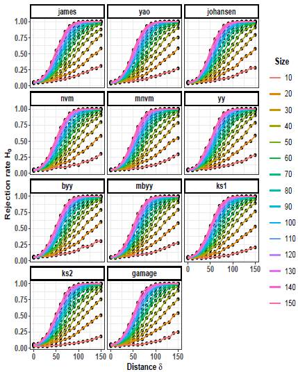
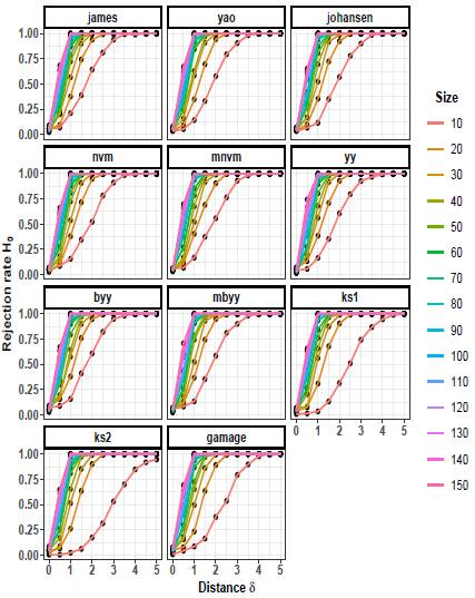
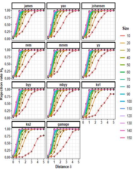
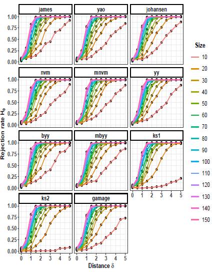
Figure 10 illustrates the behavior of the rejection rate for the hypothesis H0: μ 1 = μ 2 as a function of sample size n and δ for Yanagihara and Yuan's test when p = 3 and k = 2. In this figure, we observe the general pattern that as the sample size n or δ increases, the rejection rate also increases. This observed pattern is consistent for each test, regardless of the dimension p or the value of k.
6 Conclusion and Discussion
In conclusion, the simultation study has provided valuable insights into the performance of the R functions developed for addressing the Behrens-Fisher problem. The analysis of various factors and their impact on the rejection rates of the null hypothesis has yielded important findings.
The results indicate that as the sample size n increases, the rejection rate of H0 increases. This suggests that larger sample sizes enhance the power of the statistical test in detecting differences between the mean vectors. Consequently, the probability of correctly rejection the null hypothesis when it is false is higher, reflecting the increased sensitivity of the tests.
Another interesting finding is that as the distance δ increases, the rejection rate also increases. This is an expected result because as the distance between mean vectors increases, we anticipate a rise in rejection rates. This observation confirms that the implemented tests are functioning correctly.
We observed that as the scaling factor k increases, the rejection rate of the null hypothesis decreases. This implies that a larger scaling factor leads to a more conservative test, reducing the likelihood of erroneously rejecting the null hypothesis. However, as the sample size n increases, the rejection rate of H 0 increases regardless of the value of k.
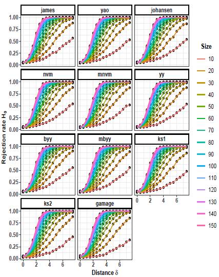
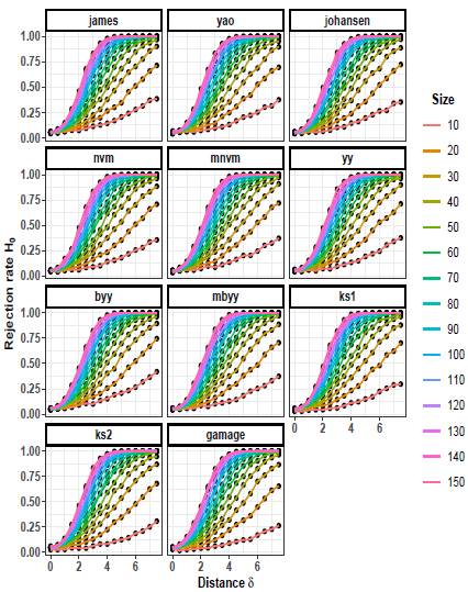
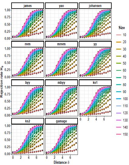
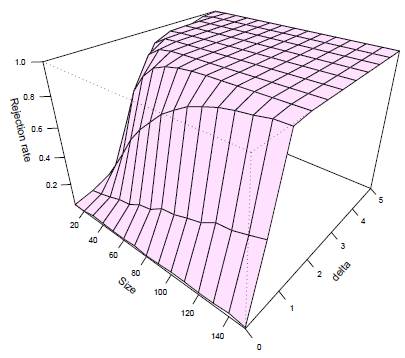
Figure 10: Rejection rate of H 0: μ 1 = μ 2 as a function of sample n and δ for Yanagihara and Yuan's test when p = 3 and k = 2.
We observed that the trajectory lines for rejection rates of H0 tend to decrease for larger values of k and small sample sizes, but these trajectories approach 100% as the sample size increases.
The developed R functions offer a user-friendly and accessible tool for conducting Behrens-Fisher tests. The simplicity and efficiency of these functions make them highly convenient for researchers and practitioners in the field. Users can confidently rely on the accuracy and reliability of these functions, as demonstrated by the comprehensive evaluation and validation carried out in this study.
In summary, the R functions developed for the Behrens-Fisher problem have exhibited robust performance, providing reliable and powerful tools for hypothesis testing. Researchers and practitioners can readily employ these functions to analyze their data, confident in their ability to accurately assess differences between mean vectors. The accessibility and user-friendliness of these functions further enhance their usability and contribute to the advancement of statistical analysis in multivariate data.

