


 Spanish (pdf)
 Article in xml format
 Article references
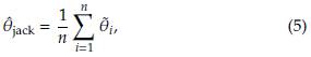
 Send this article by e-mail
 Cited by SciELO
  Cited by Google
  Similars in
SciELO
Similars in
SciELO  Similars in Google
 Permalink
1 Introduction
Two popular resampling methods widely used in real data analysis are Bootstrap [6,10] and Jackknife [24,25,31]. Both are nonparametric statistical methods. These computer-intensive techniques can be used to estimate bias and standard errors of non-traditional estimators, especially useful when the sampling distribution of an estimator is unknown or cannot be defined mathematically so that classical statistical analysis methods are not available. Samples from the observed data allow us to draw conclusions about the population of interest. Nowadays, these approaches are feasible because of the availability of high-speed computing. Confidence intervals based on Bootstrap and other resampling methods (for example, Jackknife) should be used whenever there is cause to doubt the assumptions of parametric confidence intervals. When the underlying distribution of some statistic of interest is unknown, these strategies can be beneficial.
Bootstrap and Jackknife methods are powerful techniques used in statistics to estimate the variability of a statistic or to assess the goodness of fit of a statistical model. While the Bootstrap resamples with replacement, the Jackknife method systematically leaves out one observation at a time. The choice of method depends on the problem, and both methods can be useful in different scenarios. Bootstrap and Jackknife have been used and compared in several statistical scenarios. Among others in linear regression [11, 33], quantile regression [15, 19], analysis of variance [7, 8], and generalized linear models [21]. Bootstrap and Jackknife can be used in kernel density estimation and kernel regression to estimate the variability of the density and regression functions and, consequently, define confidence intervals. In this work, we explore the applicability of these methods in the estimation of the bandwidth in both scenarios, kernel density, and kernel regression estimation. The analysis is carried out using simulated data in R [26].
The article is organized as follows: Initially, we show in Section 2 a review of the bias, standard error, and confidence intervals using Bootstrap and Jackknife. An illustration based on the coefficient of variation is also shown. In Sections 3 and 3.2, Bootstrap and Jackknife are compared in the context of hypothesis testing for one sample problems. Notably, using Monte Carlo simulations, the power of the tests based on these two strategies is estimated when testing hypotheses about the coefficient of variation are carried out. In Sections 4 and 5, we show a comparison of these methodologies in the context of kernel density estimation [5] and kernel regression [3].
2 Background: Bootstrap and Jackknife
Here we give an overview of Bootstrap and Jackknife methods. The estimations on bias and standard errors (consequently the respective confidence intervals) by both approaches are presented. Assume Y
1
, . . . ,Y
n
a random sample of Y ∼ f (y,Θ) with Θ a parameters vector that defines the probability model of interest (for example Θ = (μ, σ) in the case of a normal distribution or Θ = (α, β) for a Gamma distribution). Suppose we want to estimate
 a particular parameter (or a function of parameters) of the distribution. If the distribution of the estimator ˆθ is unknown, Bootstrap and Jackknife procedures (sections 2.1 and 2.2) can be used for obtaining a CI for θ.
2.1 Bias, standard error, and confidence intervals using Bootstrap
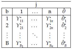
Based on the sample, we can obtain B size n samples with replacement (Table 1) denoted as Y'
bj
., with b = 1,...,B and j = 1,...,n. At each case, the estimator (
 ) of the parameter of interest is calculated.
Using the Bootstrap samples and the estimations
, b = 1,..., B in Table 1: Representation of the Bootstrap random samples: Asterisk indicates that a sample size n with replacement is obtained from
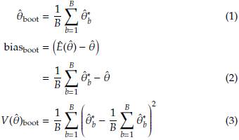
Assuming normality a 100(1 - α)% CI to 6 is given by
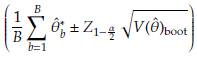
In general the CI can be obtained as
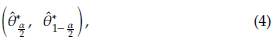
with
 and
and
 percentiles obtained from
 = 1,..., B.
2.2 Bias, standard error, and confidence intervals using Jackknife
As in the previous section, assume that we have a sample Yi,..., Y
n
be a random sample of Y ~ f(y, θ), θ is the parameter of interest and
 = g(YB,..., Y
n
) its estimator. The bias (E(
) - and the variance V(
) are unknown. Let
= g(YB,..., Y
n
) its estimator. The bias (E(
) - and the variance V(
) are unknown. Let
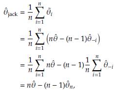
 - the estimator obtained after deleting Yi, i = 1,..., n. The Jackknife estimator of θ is defined as
where
 = n
= n
 - (n - 1)
 .
,i = 1,n, are called Tukey's pseudovalues. Alternatively we have
.
,i = 1,n, are called Tukey's pseudovalues. Alternatively we have
with

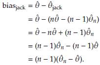
In order to estimate the bias of the Jackknife estimator, E(
 ) and θ are replaced by
and
jack respectively. Specifically
) and θ are replaced by
and
jack respectively. Specifically
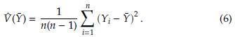
Let Y 1,..., Y n be a random sample and Ȳ the sample mean. The variance of this statistic can be approximated using the sample variance as
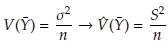
and consequently
Adapting the equation (6) to the pseudo-values
1
,...,
n
we have
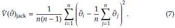
It can be shown that [9] T =
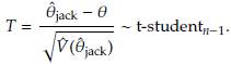
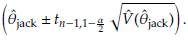
Then a 100(1 - α)% CI for θ is
3 Inference on the coefficient of variation using Bootstrap and Jackknife
In this Section, we show, using Monte Carlo simulation, the behavior of Bootstrap and Jackknife in statistical inference (estimation and hypothesis testing) on the coefficient of variation.
3.1 Estimation of the coefficient of variation
Assume Y ∼ f (y,Θ), μ = 𝔼(Y), and σ
2 = 𝕍(Y), and we want to estimate the coefficient of variation θ = CV =
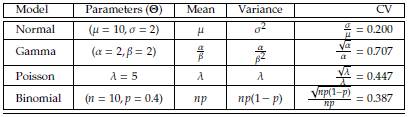
 . Based on Monte Carlo simulation [4], we compare Bootstrap and Jackknife in terms of bias and standard errors of estimation. [33] conducted a similar study based on Normal data. We extend that work using simulations from four probability models (Normal, Gamma, Poisson, and Binomial) obtained using R [26]. In Table 2, we show the expressions of the CV of the four models considered.
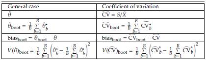
To estimate the CV using Bootstrap, we first take a random sample size n with replacement from the original dataset. We then calculate the CV of this bootstrap sample. We repeat this process B times to obtain B bootstrap samples and CV estimates. The standard deviation of these B estimates can be used as an estimate of the standard error of the CV. The confidence interval for the CV can then be obtained using the standard error and the desired level of confidence. To estimate the CV using Jackknife, we create n subsamples by leaving out one observation from the original dataset at a time. We then calculate the CV of each subsample. The mean of these n estimates is used as an estimate of the CV. To facilitate the interpretation of the results in Tables 3 and 4 are presented the expressions of Bootstrap and Jackknife estimation defined in Sections 2.1 and 2.2 corresponding to the coefficient of variation. We consider samples size n = 5,10,15,..., 200. The results are presented in Figure 1. Various aspects are remarkable in this Figure. The Jackknife bias is less than the Bootstrap one, and its performance increases with continuous distributions (Normal and Gamma). Bootstrap underestimates the CV in all cases considered. We note that the greater the sample size, the better the Bootstrap estimation (less bias). For n values close to 200, the estimations by these methodologies are very similar. The methods produce similar standard error estimations from relatively small sample sizes. The results in Figure 1 suggest that Jackknife can be a better option for estimating bias and standard deviation of the coefficient of variation, particularly when the sample size is small.
Table 2: Probability models considered to study the consistency and power of the tests on the coefficient of variation
3.2 Hypothesis testing on the coefficient of variation
The power of a test using Bootstrap or Jackknife depends on the number of resamples or Jackknife samples used, as well as the characteristics of the original dataset. Generally, increasing the number of resamples or Jackknife samples will increase the power of the test, but at the cost of computational time. An essential factor that can affect the power of the test is the underlying distribution of the data. Bootstrap and Jackknife methods can perform well if the data are normally distributed. Here, we empirically compare (using simulated data) the power of tests based on Bootstrap and Jackknife. For this purpose, we simulate samples from the distributions in Table 2. Specifically, we test the hypothesis
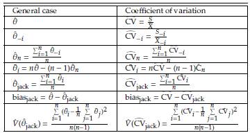
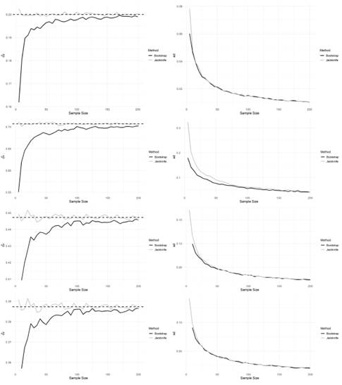
Figure 1: Estimation (left) and standard error (right) of the coefficient of variation according to the sample size (grey and black curves correspond to Jackknife and Bootstrap, respectively). The dashed line in the left panel corresponds to the CV of reference. From top to bottom, we have the results for Normal, Gamma, Poisson, and Binomial distributions, respectively.
with CV0 defined with the expressions in the last column of the Table 2. The steps to calculate the power curves for each one of the probability models considered are the following
We fix a sample size n = 100 and a significance level a = 5%.
One sample size n is simulated under the null hypothesis.
We generate many Bootstrap and Jackknife samples by resampling with replacement or deleting one observation at a time, respectively.
For each Bootstrap or Jackknife sample, the CV is calculated and used to test whether it is significantly different from the CV under the null model (given in Table 2).
The proportion of times the null hypothesis is rejected across all Bootstrap or Jackknife samples is calculated This proportion is an estimate of the power of the test.
We repeat steps 3-5 for many values of \i, a, A, and p, respectively, under the alternative hypothesis.
The results obtained are presented in Figure 2. These suggest that in all cases (four probability models), the tests based on Bootstrap are more powerful than those found with Jackknife.
4 Review of Bootstrap and Jackknife in kernel density estimation
Kernel density estimation is widely used in several applied contexts, including, among others, marine biology [22], chemistry [20], and econometrics [34]. A fundamental aspect of kernel estimation is bandwidth selection. Usually, leave-one-out and k-fold cross-validation are used for establishing the optimal bandwidth [3]. Here we compare the performance of Bootstrap and Jackknife in this scenario. Bootstrap and Jackknife can be used to estimate the variability of the kernel density estimator, but they differ in how they generate the resamples. Bootstrap requires random sampling with replacement, while Jackknife involves leaving out one observation at a time. In this section, we compare these strategies according to their performances in both histogram density estimation (Section 4.1) and kernel density estimation (Section 4.2). Specifically, we estimate the uncertainty of the estimated density function in kernel density estimation.
4.1 Bootstrap and Jackknife in bandwidth histogram estimation
The histogram is one of the most broadly used graphical tools in descriptive data analysis [29]. This tool is a kernel density estimator where the underlying kernel is uniform [3]. Although there are better options for estimating the density, in this work, we consider the histogram given its extensive use in real data analysis. Specifically, it is established which of the two resampling methodologies (Bootstrap or Jackknife) performs best in estimating the amplitude of the class intervals.
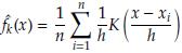
Given an observed sample X1, x n , the histogram estimator of the density function f (x) is defined as
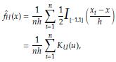
With
The optimal bandwidth h is the one that minimizes the asymptotic mean integrated squared error (AMISE), defined as [3]
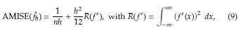
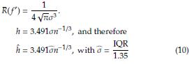
where f(x) is the population density. To estimate h is usually considered f(x) as a Gaussian distribution with mean and standard deviation estimated from the sample. Taking derivative of the AMISE with respect to h and equating to zero yields

Under the Gaussianity assumption
4.2 Bootstrap and Jackknife in bandwidth kernel density estimation
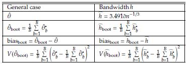
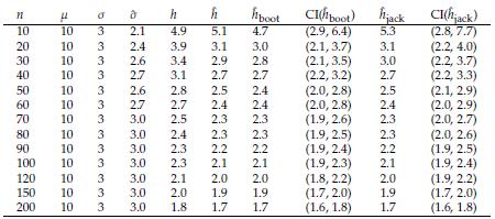
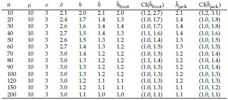
The problem of estimating h depends only on the j estimation. Here we evaluate the performance of Bootstrap and Jackknife in the estimation of h. The estimations obtained are compared with the classical estimation given in Equation (10). The Tables 5 and 6 show in parallel the general definitions of Bootstrap and Jackknife estimators and the corresponding expressions for estimating the bandwidth h by means of these approaches. In order to compare the methodologies, we conduct a simulation study. Suppose X ~ N ( μ= 10, σ = 3). Using R software [26], we simulate random samples size n = 10,20,30,..., 200 from X, and at each case, we estimate the parameter h by using the estimator in Equation (10). We also carry out an estimation of h through Bootstrap and Jackknife (see Tables 5 and 6). The simulation results are shown in Table 7. There are several remarkable aspects of this Table.
Table 5: Summary of Bootstrap estimation of the bandwidth h in kernel density estimation. Assume that ĥ * b is the estimation of the bandwidth h based on a Bootstrap sample
With small samples, the estimations by the three methods (classical, Bootstrap, and Jackknife) are very similar, and for large samples (n ≥ 60), the three estimations coincide. In all cases, the estimations are very close to the value of the parameter h. This result indicates that any of them can be used. However, one advantage of Bootstrap and Jackknife over classical estimation is that these allow for assessing the uncertainty of the estimations (employing the corresponding confidence intervals). As expected with both methodologies (Bootstrap and Jackknife), a large sample size provides narrower confidence intervals. In all cases, Bootstrap and Jackknife confidence intervals contain the corresponding parameter h. The results indicate that Bootstrap and Jackknife are valid and valuable alternatives for estimating the interval bandwidth in the histogram density estimation. These are preferable to the classical estimation since they allow obtaining, in addition to the point estimation, a measure of variability in the estimation. In the case of small samples, the Bootstrap intervals are slightly narrower than those obtained with Jackknife. This point suggests that Bootstrap might be more suitable when n values are small. Let x1,..., xn a sample size n of a population with unknown density(
 (x)) The kernel density estimator of f (x) is given by
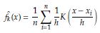
where K is a kernel function (Gaussian, Epanechnikov, triangular, biweight, etc.) and h is the bandwidth. The optimal h is the value that minimizes the AMISEf (x)) defined as
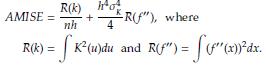
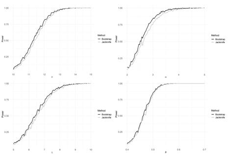
Figure 2: Power curves based on simulated data. One side hypothesis of the coefficients of variation obtained with four probability models. Normal (μ = 10, σ - 2) (top left), Gamma(α - 2,β - 2) (top right), Poisson (λ - 5) (bottom left), Binomial (n - 10, p - 0.4)
Table 6: Summary of Jackknife estimation of the bandwidth h in kernel density estimation. Assume that σ-i is the estimation of standard deviation based on a sample x ¡-1 , x ¡+1 ,…x n .
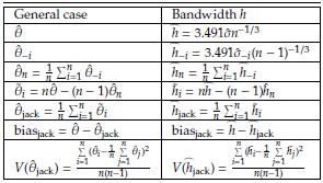
Table 7: Assume X ~ N(/μ, o). h: optimal amplitude in histogram density estimation. h: classical estimation. ĥ boot and ĥ jack are the approaches based on Bootstrap and Jackknife, respectively. In these cases we also include 95% confidence intervals.
Estimator of f(x) is given by
where K is a kernel function (Gaussian, Epanechnikov, triangular, biweight, etc.) and h is the bandwidth. The optimal h is the value that minimizes the AMISE(
 (x)) defined as
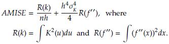
Table 8: Assume X ~ N(μ, σ). h: optimal amplitude in kernel density estimation. h: classical estimation. ĥ boot and ĥ jack are the approaches based on Bootstrap and Jackknife, respectively. In these cases we also include 95% confidence intervals.
Differentiating the AMISE with respect to h we have
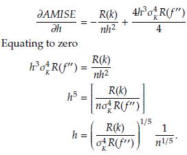
The optimal bandwidth h is obtained assuming f (x) as a Gaussian density. Hence, after some calculations, we have that the optimal bandwidth in kernel density estimation is obtained by
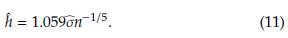
Changing ĥ - 3.491ôn-1/3 by Equation (11) in Tables 5 and 6, we obtain the corresponding expressions to do the estimation of the optimal bandwidth in kernel density estimation by using Bootstrap and Jackknife. In Table 8, we show the estimations of the optimal bandwidth in kernel density estimation based on the same samples simulated to generate the results in Table 7. As in the particular case of the histogram, the bandwidth estimations shown in Table 8 indicate that Bootstrap and Jackknife can be favorable alternatives to carry out the estimation of the density using the general methodology based on kernel. We present the results using a Gaussian kernel; however, we obtained similar results with others. As in the case of the histogram estimation, in this section, we can conclude that using Bootstrap or Jackknife can be preferable because these approaches allow having an estimation of the variability for the estimator. Particularly with small sample sizes is helpful to know the uncertainty in the estimation. As in the case of the histogram estimation, we note that Bootstrap can be preferable with small samples because narrower confidence intervals are obtained. The results in Tables 7 and 8 show that the estimators ĥ boot and ĥ jack are consistent, i.e, limn→∞ ĥ boot - h and lim n→∞ ĥ jack = h.
5 Bootstrap and Jackknife in bandwidth kernel regression estimation
Bootstrap and Jackknife have been compared under various regression contexts. Among others in linear [2], generalized linear [12, 30, 33], and logistic regression [14]. This paper compares the efficiency of Bootstrap and Jackknife in estimating the bandwidth in kernel regression. This parameter, denoted as h (as in Sections 4.1 and 4.2 but now in a regression scenario), determines the width of the kernel function, which in turn affects the smoothness of the estimated regression function. The choice of the bandwidth is critical, as it can greatly affect the bias and variance of the regression estimator. Suppose we have an observed bivariate random sample (y i, x i), i = 1,..., n with y and x the response and predictor variables, respectively. We want to estimate the regression model.
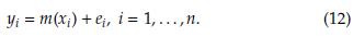
Let f(x) and f(x, y) be the univariate and bivariate density functions of the variable X and the random vector (Y, X). The estimation of a kernel regression model based on the observed sample (x i , y i ), i = 1,..., n is given by [3]
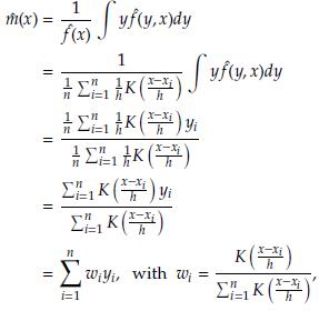
where K is a kernel (Gaussian, rectangular, triangular, Epanechnikov, etc) and h > 0 is the bandwidth that controls the amount of smoothing. For a particular i, i - 1,..., n, we have
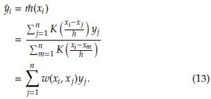
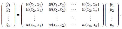
In matrix notation, the estimates at the n sampling points are calculated as
A key point in kernel regression is to determine the bandwidth h. The usual strategy is based on choosing the h value that minimizes the mean squared error (MSE) defined as [18]
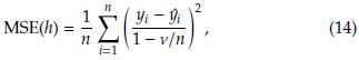
with
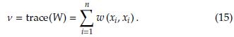
In general, a small bandwidth will result in a high degree of local smoothing, while a large bandwidth will lead to less local smoothing and more global effects. A bandwidth that is too small may generate overfit of the data, while a bandwidth that is too large may produce an over-smoothing of the data and miss significant local trends. Various methods can be used to determine the optimal bandwidth, such as cross-validation or minimizing a particular criterion (e.g., mean squared error or Akaike's information criterion). Cross-validation involves partitioning the data into training and validation sets and evaluating the performance of the model with different bandwidth values. The bandwidth that results in the best behavior on the validation set is then chosen as the optimal bandwidth. In this Section, we compare Bootstrap and Jackknife to establish their efficiency in estimating the optimal bandwidth h in kernel regression according to the criterion in Equation (14). The Jackknife method in kernel regression involves repeatedly fitting the kernel regression estimator to a subset of the data, leaving out one observation each time. The estimation of the kernel regression function is then calculated using all the observations and each subset of the data. The Jackknife estimation of the bandwidth is obtained using the pseudovalues are calculated as
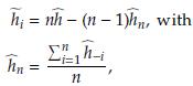
where ĥ and ĥ -1 are defined using the criterion in Equation (14), with and without considering, respectively, the i-th observation (y i, x i), i - 1,..., n. The pseudo-values can be used to estimate h, the variance of the kernel regression estimator h and a confidence interval for h. Specifically we have
Using the quantiles
 and (1-
) from the pseudovalues, an approximate confidence interval for the bandwidth of the kernel regression can be obtained as
and (1-
) from the pseudovalues, an approximate confidence interval for the bandwidth of the kernel regression can be obtained as

On the other hand, the Bootstrap method can also be used to obtain many estimations (using resampling with replacement) and, consequently, a variability measure and a confidence interval for the bandwidth h calculating the quantiles of the distribution of the Bootstrap estimations. Let (x* 11, y* 11),… (x * 1n, y * 1n),… (x * B1, y* B1),… (x * Bn, y * Bn) be B Bootstrap samples size n taken from (x i, y i), i = 1,..., n. Based on each one of these is obtained an estimation of h according to the criterion in Equation (14), i.e., we find (ĥ* 1,..., ĥ* b). The Bootstrap estimator of the bandwidth, its variance, and the corresponding confidence interval are given by
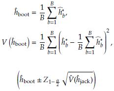
Using the quantiles of the Bootstrap estimations (ĥ* 1,..., ĥ* B ) a confidence interval for the bandwidth of the kernel regression estimator can be also obtained as

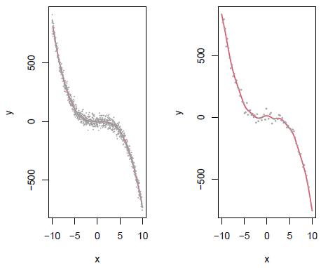
Figure 3: Left panel: Scatterplot of (x i, y i), i = 1,..., 1000 points simulated from the model Y - 0.2x + 0.5x2 - 0.8x3 + ∈, ∈ ~ N(0,30) which is assumed as the population data and fitted kernel regression model with h - 0.37 (red curve). Right panel: Simulation of n - 80 data from the population data (gray points in the right panel) and estimated kernel regression model (red curve) with ĥ= 0.65.
5.1 Simulation study
Here we present some simulation results comparing Bootstrap and Jackknife in estimating the bandwidth in kernel regression. For this purpose we assume Y - 0.2x + 0.5x2 - 0.8x3 + e, e ~ N(0,30) as the population model (Figure 3). The red line corresponds to the fit of a kernel regression model with bandwidth h - 0.37, which was calculated according to the criterion in Equation (14). The comparisons are made by taking samples of size n - 20,40,60,..., 200 from this model. For illustrative purposes, in the right panel is presented an estimated a kernel regression model with a sample size n 80 of the population model. In this case, the bandwidth estimation is ĥ =0.64. Varying the sample size are obtained the estimations h, hboot and ĥ jack (Table 9). Note that in practice given a dataset (xi, yi), i = 1,..., n we have just one estimation of h and several estimations of ĥ boot and ĥ jack obtained by resampling the data recorded. In this real case, we only could determine confidence intervals employing the approaches based on Bootstrap and Jackknife. For this reason, in order to compare the three methodologies (classical, Bootstrap, and Jackknife), we calculate confidence intervals based on the percentiles 5% and 95% obtained from 300 sets of values of ĥ, ĥ boot and ĥ jack generated with an equal number of samples size n - 20,40,60,..., 200 simulated from the population model (Table 9). The results suggest that the tree estimators are consistent, i.e., as we collect more and more data (when n increases), the difference between the estimated value and the "true value of the parameter " (assumed equal to 0.37) will become smaller and smaller. According to the results in Table 9, the Jackknife estimations are very close to the obtained with the classical approach. We also note (see last row of the table) that the estimates by Jackknife tend more quickly to the fixed reference value (ĥ = 0.37) than those obtained by Bootstrap. These results indicate that Jackknife may be a more appropriate and efficient option than Bootstrap to estimate the bandwidth in Kernel regression. In general is accepted that in regression problems, as long as the data set is reasonably large, Bootstrap is often acceptable. However, the estimations ĥ boot and the corresponding confidence intervals CI(hboot) in Table 9 suggest that in the context of Kernel regression, Bootstrap is not the best option to establish the variability of the bandwidth estimator ĥ.
Table 9: Assume Y - 0.2x + 0.5x2 - 0.8x3 + ∈ a regression function with e ~ N(0,30). The optimal bandwidth (see Section 5) in a kernel regression model calculated with 1000 data simulated from the population model is h - 0.36. ĥ, ĥ boot, and ĥ jack identify the approaches classical and based on Bootstrap and Jackknife, respectively, which are calculated for each sample size as the mean of fifty simulations. We also include 95% confidence obtained as percentiles 5% and 95% of the fifty estimations.
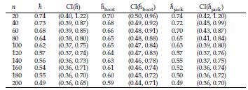
Table 10: Results based on Bioluminescence data. Assume Y m(x)+e, with m(x) a kernel regression function. ĥ: optimal estimation based on lest square. ĥ boot and ĥ jack are the approaches based on Bootstrap and Jackknife, respectively. In these cases, we also include 95% confidence intervals.
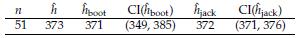
Figure 4: Scatterplot (dots) of pelagic bioluminescence along a depth gradient in the northeast Atlantic Ocean for a particular station. Data taken from [35]. Red curve corresponds to a Kernel regression model with an optimal bandwidth h - 373.
5.2 Application to bioluminescence data
Bioluminescence is the emission of light by living organisms, typically due to chemical reactions involving luciferin and luciferase enzymes [16]. Overall, analyzing bioluminescence data can provide valuable insights into the biological processes and respect for the environmental and experimental factors affecting bioluminescence activity [27]. Bioluminescence is very common in the ocean, at least in the pelagic zone. Bioluminescent creatures occur in all oceans at all depths, with the greatest numbers found in the upper 1000 m of the vast open ocean [32]. The relationship between pelagic bioluminescence and depth has been considered from various perspectives. Among additive models [13], [17], and additive mixed models [36] have been used in this context. This work applies a Kernel regression model to a pelagic bioluminescence dataset taken from [35]. Based on these data, the aim is to illustrate how to define confidence intervals for the bandwidth h parameter. The scatterplot and the fitted Kernel regression model with bandwidth h - 373 are shown in Figure 4
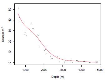
Figure 4: Scatterplot (dots) of pelagic bioluminescence along a depth gradient in the northeast Atlantic Ocean for a particular station. Data taken from [35]. Red curve corresponds to a Kernel regression model with an optimal bandwidth ĥ = 373.
From Table 10, we can establish that the optimal bandwidth h that minimizes the criterion in Equation (5) is ĥ - 373. We also note that the estimations by Bootstrap and Jackknife are very close to this value; however, Jackknife is a better option to define the confidence interval for h because, on the one hand, it includes the h value and, on the other hand, is shorter than the obtained by Bootstrap. The results in this Section confirm that Jackknife is a good alternative in kernel regression to define the bandwidth estimation uncertainty.
6 Conclusion and further research
The results in this work suggest that in the particular case of the coefficient of variation, Jackknife tends to produce less biased estimates, but it may have lower power than Bootstrap. In the case of the histogram and kernel density estimation, both methodologies produce similar results. Finally, in the context of Kernel regression, Jackknife is a better option. Resampling methods are helpful nowadays in many contexts. Power studies comparing these approaches in many statistical areas are required. For example, evaluating its performance in splines regression and neural networks can be valuable.

