


 text in
  English (pdf)
 Article in xml format
 Article references
 Send this article by e-mail
 Cited by SciELO
  Cited by Google
  Similars in
SciELO
Similars in
SciELO  Similars in Google
 Permalink
INTRODUCTION
Malpelo Island and its surrounding marine area are home to a great species richness, leading to its worldwide recognition as a biodiversity “hotspot”. Because of this, in 1995 the Colombian government reserved, delimited, and declared Malpelo Island a protected area, with the category of Fauna and Flora Sanctuary (FFS) (Ministry of the Environment, 1995), integrating it into Colombia’s National Natural Park System. Since its declaration, the protected area has been extended four times (1996, 2002, 2005, and 2017). Currently, it has an area of 2,667,908 ha (Ministry of Environment and Sustainable Development, 2017), of which only 63.3 ha correspond to the emerged area (Malpelo Island and 12 islets).
Due to its location in the central part of the Panama Bight (PB), the waters of the Malpelo FFS are of great importance from an oceanographic point of view, since they are located in an area of confluence between the cold waters of the south of the PB and the warm waters of the north of the PB. The Sanctuary covers a considerable part of the Malpelo Ridge, a geomorphological structure of great biophysical complexity along which processes and phenomena of great significance occur, justifying its identification as an Ecologically or Biologically Significant Marine Area (EBSA). The PB is an area of considerable interest because it marks the eastern limit of the waters of the Equatorial Counter Current, and because it displays strong interannual variability associated with the El Niño Southern Oscillation (ENSO) (Fiedler and Talley, 2006). Due to its position in the low-pressure equatorial concavity, the PB is strongly influenced by the Intertropical Convergence Zone (ITCZ), since this modulates the annual cycle of oceanographic and hydroclimatic conditions in the region (Forsbergh, 1969) and generates mesoscale processes that in turn directly influence the climate of the PB and of the Malpelo FFS, such as the winds of the Panama jet (Chelton et al., 2000; Amador et al., 2006; Rodríguez-Rubio and Giraldo, 2011). As a result, a seasonal upwelling event occurs between December and March in the Gulf of Panama and the central portion of the PB, where the Malpelo FFS is located, which generates a decrease in Sea Surface Temperature (SST) and an increase in chlorophyll-a (Chl-a) concentrations (Legeckis, 1986; Rodríguez-Rubio and Stuardo, 2002). During this period, SST values of 26.0 to 27.5 °C are recorded for the sanctuary, alongside salinities between 32.0 to 33.0 (Rodríguez-Rubio et al., 2007). However, towards the western margin of the Malpelo FFS, SST values above 27.5 °C and salinities of 32.0 and 32.8 are observed (CCO and Dimar, 2019). During the rest of the year the wind field is dominated by southerly trade winds that limit the development of oceanic upwelling (Kessler, 2006). During the second half of the year, SST presents a smaller gradient of change than that observed during the January-April period, where the majority of SST values are between 27.0 to 27.2 °C and salinities fall between 32.0 and 32.2 (CCO and DIMAR, 2019).
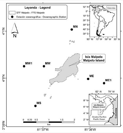
In order to produce inputs that would help it manage the sanctuary, the Pacific Territorial Direction (DTPA in spanish), initiated a process to monitor oceanographic conditions in the area in 2006. This work has been supported by the Universidad del Valle since 2012. Monitoring has been carried out continuously from that date until the present year (2021), with the exception of 2018, resulting in a total of 15 years of sampling. The sampling network currently used consists of six stations located 0.93 km (0.5 nautical miles) and 1.85 km (1 nautical mile) from the island. This design is presumed to be inefficient, due to the small distances between stations, and insufficient, given the large size of the sanctuary (26,679 km2). The northwestern vertex, which limits with the Yurupari Malpelo National Integrated Management District (DNMI), is 124.08 km (67 nautical miles) from the island, while the northeastern limit, the most distant, is 172.24 km (93 nautical miles) away. Given the current need to reformulate the oceanographic sampling network to ensure it is capable of providing the best possible information and is cost-effective, the objective of this paper is to design an optimal sampling network based on an analysis of the spatial autocorrelation structure of SSTs in the Malpelo FFS, using geostatistical analysis for data gathered in situ and from remote sensors.
MATERIALS AND METHODS
Study area
The Malpelo FFS is located in the central section of the Colombian Pacific Basin (CPB) (Figure 1), itself contained within the Panama Bight (PB), which in turn forms part of the Eastern Tropical Pacific (ETP). Malpelo Island is located in the center of the sanctuary, which itself occupies the westernmost portion of Colombia’s land territory in the Pacific. It is separated from the continental territory by more than 380 km and located approximately 505 km west of the port of Buenaventura (Department of Valle del Cauca, Colombia) of which it forms a part. The island is elongated in shape, with a length of about 1,643 m; it is of variable width (maximum 727 m) and reaches a height of 300 m. There are 12 islets in the surrounding waters. The emerged portion of the islands (Malpelo and the islets) has an area of about 0.633 km2. However, its three-dimensional surface is about 1,215 km2 (López-Victoria and Rozo, 2006).
Data sets
Two data sets were used for the spatial variability analysis of SST in the Malpelo FFS: one obtained in situ and the other derived from a MODIS-Aqua (Moderate Resolution Imaging Spectroradiometer-Aqua) sensor. Surface temperature is a variable that has been used in the design of sampling networks such as the one proposed by Giraldo et al. (2001) for the estuary of the “Ciénaga Grande de Santa Marta”, Colombia. Further, to demonstrating that the technique fitted a semivariance model easily, this study showed temperature to be a cost-efficient variable and therefore suitable for formulating sampling networks using geostatistical analysis of spatial autocorrelation. The data obtained in situ corresponded to the oceanographic monitoring carried out by the DTPA between 2012 and 2019 with support from the Universidad del Valle. During this period, thirteen sampling were carried out with a periodicity of between one and three samplings each year. The network sampling employed consists of six stations located around the island at distances of between 0.93 km (0.5 nm) and 1.83 km (1 nm) (Figure 1). The second dataset was obtained using the MODIS SST v2019 product, derived from the MODIS-Aqua sensor (Werdell et al., 2013). The time period used was July 2002-July 2019 (205 months/17.1 years). The images used were global, with a processing level L3, taken by the sensor during the day, with a monthly temporal resolution and a spatial resolution of 4 km. SST data derived from longwave infrared thermal bands at 11 µm and 12 µm (bands 31 and 32) were employed. These data sets are distributed by the Physical Oceanography Distributed Active Archive Center (PO.DAAC) (https://podaac.jpl.nasa.gov). Information was extracted from the Malpelo FFS polygon for each month.
Statistical analysis
When multiple regionalized variables are available (in this case in situ and remotely sensed SST) an alternative way to address the multivariate problem is to use a Principal Component Analysis (PCA) (Giraldo, 2002). This technique is widely used to partition the variance of a set of spatially distributed time series into a few uncorrelated statistical modes, or Principal Components (PC). PCA involves the calculation of Empirical Orthogonal Functions (EOF), which may be described as a set of vectors that maximize the variance of the variables used and constitute the orthogonal basis of a set of time series at different measurement sites. After generating the principal axes in the traditional way, following Manly and Navarro (2016), these were then interpreted in terms of the variability explained by each component with respect to each original variable; finally, a geostatistical analysis was carried out by estimating the semivariance function and applying a Kriging procedure using the data taken from the axes generated (Giraldo, 2002).
For the in situ sampling, the PCA sampling units used were the stations of the Malpelo FFS oceanographic monitoring network (six stations) and the variables were the sampling performed (13). The sampling units used for the remote sensing SST analysis were the pixels in each SST image of the Malpelo FFS (1284), while the variables were the months of the entire series (July 2002-July 2019). A correlation matrix (Emery and Thompson, 2014) was used to derive the eigenvectors and eigenvalues. The numerical analysis of the in situ data was performed using the Statistica v7.0 program (Statsoft, 2007) and the analysis of the remotely sensed data was based on imagery and performed using the “Principal Components” tool contained in the ArcGis 10.5 software. Subsequently, geostatistical analyses were performed using the maximum variance component (Principal Component 1, or PC1).
One of the important applications of the study of georeferenced information using geostatistical analysis is the design of sampling networks (Cressie, 1989). The first stage in the development of a geostatistical analysis is the determination of the spatial dependence between the measured data of a variable. Three functions may be used to carry this out: the semivariogram, covariogram and correlogram (Giraldo, 2002). Of these, the only function that does not require parameter estimation is the semivariogram or dissimilarity function, and it was therefore chosen to analyze the spatial correlation structure of SST in the Malpelo FFS.
The semivariance function characterizes the spatial dependence properties of the process being evaluated. This function is calculated for various distances, h. To interpret the experimental semivariogram, it is assumed that the smaller the distance between sites, the greater the spatial similarity or correlation between observations. Therefore, in the presence of autocorrelation, it is expected that for small values of h the experimental semivariogram will have smaller magnitudes than those it takes when the distances h increase. Since the experimental semivariogram is calculated only for some average discrete distances, it is necessary to fit models that generalize the observed experimental semivariogram to any distance. In general such models can be divided into unbounded (linear, logarithmic, potential) and bounded (spherical, exponential, Gaussian) (Warrick et al., 1986). Models belonging to the second group ensure that the covariance of the increments is finite, so they are widely used when there is evidence of good fit. According to Giraldo (2002), these models have three common parameters (Figure 2), which are described below:
Nugget effect: The Nugget effect is denoted by C0 and represents a point discontinuity of the semivariogram at origin (Figure 2). It may be the result of measurement errors in the variable or to its scale. Sometimes it may be indicative that part of the spatial structure is concentrated at distances below those observed.
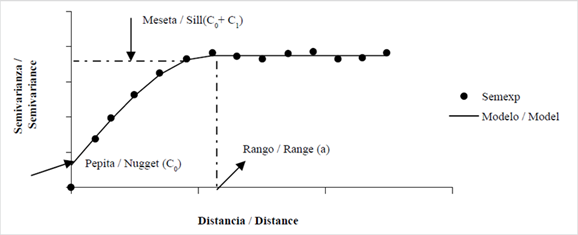
Figure 2 Typical behavior of a bounded semivariogram with a representation of the basic parameters. SEMEXP corresponds to the experimental semivariogram and MODEL to the fit of a theoretical model (Taken from Giraldo, 2002).
Plateau: The Plateau is the upper limit of the semivariogram. It may also be defined as the limit of the semivariogram when the distance h tends to infinity and there is no further spatial correlation between the sampling points. The plateau may or may not be finite. Semivariograms with finite plateaux comply with the strong stationarity hypothesis. When the opposite occurs, the semivariogram defines a natural phenomenon that complies only with the intrinsic hypothesis. The plateau is denoted by C1, or by (C0 + C1) when the nugget is different from zero.
Range: In practical terms, Range corresponds to the distance beyond which two observations are independent and not spatially autocorrelated. The range is interpreted as the zone of influence. In some semivariogram models there is no finite distance for which two observations are independent. Therefore, the distance for which the semivariogram reaches 95 % of the plateau is called the effective range. The smaller the range, the closer to the spatial independence model.
The PC1 was used to analyse the spatial autocorrelation structure using the semivariogram, since this has the highest variance and captures the greatest temporal variability of the data set. Adjustment of the PC1 models of the SST in situ and as derived from remote sensors in the Malpelo FFS, was carried out by estimating ordinal and weighted least squares. The models used were: exponential, Gaussian and spherical. Prior to this, it was verified whether the correlation presented directionality (isotropy or anisotropy). The analysis of correlation directionality, experimental semivariograms and model-fitting were performed using the GeoR routine of the R software (Ribeiro and Diggie, 2018). Mean squared error was used as a criterion to select the best model. Subsequently, using the best semivariance model, the predictions of the variable for each sampling network were performed using a Kriging method, and the variance of the prediction error was calculated for each network size using the approximation of Cressie (1993). For greater detail, Giraldo (2002) summarizes the theory of spatial autocorrelation structure estimation, the Kriging prediction method and the calculation of the variance of prediction error.
RESULTS
Data sets
During the period April 2012 to May 2019, the average in situ SST obtained in the waters of the Malpelo FFS was 26.89 °C. During the first quarter of the year (January-March) the average temperature was 25.57 °C, during the second (April-June) 28.08 °C, during the third (July-September) 27.38 °C and during the fourth (October-December) 26.07 °C. During the 13 sampling conducted in the same period, the maximum SST levels were found in April 2012 (28.93 °C) and in September 2015 (28.58 °C). In the first case, these temperatures coincided with the end of a La Niña period (2010-2012) and in the second with the 2015-2016 El Niño. On the other hand, the minimum SST values were observed in December 2012 (23.97 °C) and March 2015 (25.11 °C) (Figure 1). In the first case, these temperatures coincided with a neutral period and in the second with El Niño 2015-2016.
The average SST at Malpelo Island obtained using the MODIS-Aqua sensor (2002-2019) was 27.11 °C. During the first quarter of the year (January-March) the average temperature was 26.78 °C, in the second (April-June) 27.75 °C, in the third (July-September) 27.03 °C and in the fourth (October-December) 26.89 °C. In the period 2002-2019, the maximum SSTs were found in May 2016 (30.17 °C) and April 2010 (29.25 °C). The first case coincided with the end of El Niño 2015-2016 and the second with the end of El Niño 2009-2010. On the other hand, the lowest SST were observed in August 2010 (23.74 °C) and March 2009 (24.01 °C) (Figure 2). In the first case, these temperatures coincided with La Niña 2010-2012 and in the second with La Niña 2009. For the Malpelo FFS polygon (grey line in Figure 2), the average SST during the period 2002-2019 was 27.23 °C. During the first quarter of the year (January-March) the average temperature was 26.72 °C, during the second quarter (April-June) 27.98 °C, during the third quarter (July-September) 27.18 °C and during the fourth quarter (October-December) 27.03 °C.
In the PCA of in situ SST, the PC1 made a contribution to the total variance of 88.3 %, with an associated eigenvalue of 5.3, while the PC2 contributed 5.4 %, with an eigenvalue of 0.3. In the analysis of SST derived from remote sensing, the PC1 contributed 65.1 % to variance with an associated eigenvalue of 21.9, and the PC2 a contribution of 12.3 % and an eigenvalue of 7.6. In terms of time, the PC1 of the remote sensing analysis described the variability of the annual cycle of SST in the sanctuary and, spatially speaking, presented a strong correlation with SST (r = 0.86; p > 0.05) (Figure 3). The north-western zone presented extreme above-average standardized values, while in the southeast the values were below average (Figure 3). In both cases (in situ and remote sensing of data), the first component accounted for a high percentage of the temporal variability, so a semivariance model was only adjusted to the first component. The calculation of the semivariance in different directions showed them to have similar shapes, so the phenomenon was considered to be isotropic.
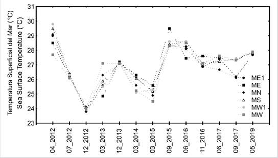
Figure 3 Sea surface temperature (SST) at the stations in the current sampling network of the Malpelo Fauna and Flora Sanctuary, recorded between April 2012 and May 2019.
When the exponential, Gaussian and spherical ordinal least squares and weighted least squares models were fitted to the in situ data (Figure 4), semivariance was very small (plateau) and in all cases the mean squares of the error were equal to zero.
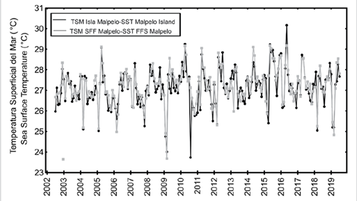
Figure 4 Sea surface temperature (SST) between July 2002 and July 2019, for Malpelo Island and the Malpelo Flora and Fauna Sanctuary polygon, obtained using the MODIS-Aqua sensor.
When fitting the exponential, Gaussian and spherical ordinal least squares and weighted least squares models to the remotely sensed data, the fitted semivariance models showed a strong spatial autocorrelation for SST. The best fitting model (lowest value of error mean squares) was found to be the Gaussian model calculated using ordinal least squares (Table 1, Figure 5). This model presented a plateau of 73.2 (maximum dissimilarity) and a range of 179,340 m.
Table 1 Theoretical semivariance models fitted to experimental semivariograms calculated for SST values obtained from the MODIS-Aqua remote sensor.
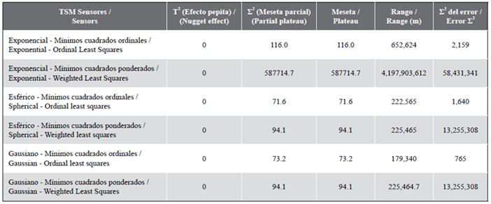
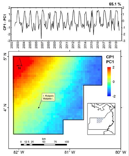
Figure 5 First standardized principal component (PC1) of a principal component analysis of Sea Surface Temperature (SST) in the Malpelo Flora and Fauna Sanctuary, using data derived from the MODIS-Aqua sensor (2002-2019).
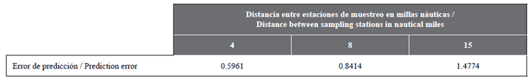
The Gaussian model obtained using ordinal least squares from remote sensing SST analysis (the best fitting model), showed that 100 % of the dissimilarity occurred when semivariance was equal to 73.2 and the range was 179,340 m. Semivariance may also be interpreted as a dissimilarity distance. For example, for the fitted Gaussian model, a dissimilarity of 20 % was found at 28.57 km (15.43 nautical miles) (Table 2). To choose the ideal distance between stations, logistical issues must also be considered, as a sampling network with stations that are too far apart and too distant from Malpelo Island would require long journeys that might be beyond the capabilities of the type of vessels that regularly carry out oceanographic monitoring in the Malpelo FFS, and the logistics associated with such sampling would be complicated. For example, a sampling network with a shape similar to the current one (Figure 1) and a distance between stations of 27.78 km (15 nm) (currently the distance between stations is between 0.5 and 1 nm) and with only eight stations (two on each axis; north-south, west-east), would take more than 38 hours to complete at an average speed of 11 km/h (6 knots). Currently, oceanographic monitoring of the Malpelo FFS is principally carried out using dive ships, which have logistical restrictions that hinder long journeys, because they also carry out other monitoring and research activities. It is therefore necessary to adopt a sampling network with shorter distances between stations. An additional criterion for choosing the gaps between stations is the prediction error (Table 3). An evaluation of this parameter in sampling networks at three different distances (27.78, 14.82 and 7.41 km - 15, 8 and 4 nm) found that it increases exponentially as a function of the distance between sampling points, and was in all cases less than 2 %. However, the sampling network with stations every 7.41 km (4 nm) returned the lowest prediction error. This value is close to that obtained in Table 2, in which the semivariance model presents a dissimilarity between stations of 5 % (7.14 km, 3.86 nautical miles).
Table 2 Distance associated with discrete values of dissimilarity, obtained using the Gaussian semivariance model of SST in the Malpelo FFS.
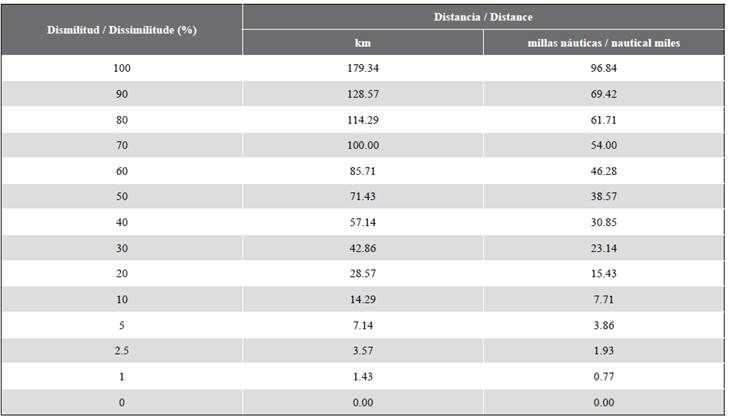
Table 3 Maximum prediction variance of Sea Surface Temperature (SST) obtained from the MODIS-Aqua remote sensor in different sampling networks, with the following distances between stations: 7.41 km (4 nautical miles), 14.82 km (8 nm) and 27.78 km (15 nm).
Thus, if a distance between stations of 7.41 km (4 nm) is used (the distance with the smallest prediction error) the sampling network for the entire sanctuary area would contain 598 stations, which from a logistical point of view would be difficult to achieve. If the limitations associated with logistics and travel distance are considered, and areas of influence established around the island of 9.26 km (5 nm) and 18.52 km (10 nm) -corresponding to the first two sampling rings of the 598-station network- is obtained a network consisting of 8 and 24 stations, respectively (Figure 6). Although other additional sampling rings could be included, this proposal has not considered them because the next ring of 27.78 km (15 nm) would include 48 stations, implying distances and logistical challenges that current conditions would render untenable. Additionally, it should be borne in mind that the Malpelo area is subject to the powerful influence of the PB current system. According to Metoceanica (2017), during the first quarter of the year, the waters of the Malpelo FFS are dominated by northeast-southwest currents, while during the third quarter the pattern is northwest-southeast. In other words, the station location axes should have an inclination of 45° and -45°, forming an “X”, so that sampling and/or monitoring can capture the variability generated by current patterns.
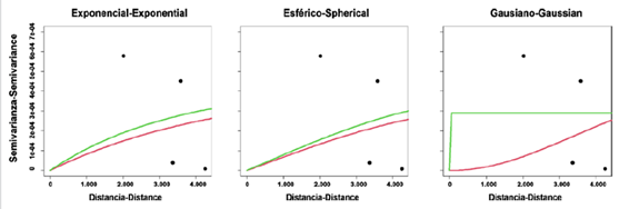
Figure 6 Experimental semi-variogram (dots) and fitted models (red line: ordinal least squares, green line: weighted least squares) for the in situ SST data of the Malpelo FFS. Distances are given in meters.
Starting from a proposed 24 stations (Figure 6) centred on the island, and selecting only the stations on the displacement axes of the currents, a sampling network of eight stations is obtained (Figure 7), producing a dissimilarity between stations close to 5 %, a prediction error of less than 1 % and an arrangement that responds to the logistical and range limitations of the vessels that regularly carry out oceanographic monitoring in the Malpelo FFS. Therefore, the proposed sampling network includes eight new stations and proposes maintaining the six stations that have historically been used for oceanographic monitoring, for a total of 14 stations (Figure 7). However, the number of existing stations retained could be reduced from six to four, by preserving only those closest to the displacement axes of the currents (MS, ME1, MN, and MW1). Due to the short distances between the stations in the current sampling network, the positions at which sampling has been historically performed do not coincide where in which the station should have been madepositioned (Figure 1). It was therefore, was necessary to adjust the station positions according to the most frequent position in which each station was realizedestablished during the period 2012-2019. These were relocated as shown in Figure 7. Table 4 presents these positions using geographic and plan coordinates (WGS84 reference system and MAGNA Colombia West, respectively), setting out the optimal sampling network of 14 stations for monitoring oceanographic conditions in the Malpelo FFS. By superimposing a SST image derived from the MODIS-Aqua sensor (July 2019) and performing a virtual sampling procedure for the stations of the old network (n = 6) and of the one proposed here (including the old stations; n = 14), it is found that for the old network the average is 27.54 °C, the range (maximum value minus minimum value) is 0.26 °C, standard deviation is 0.12 and the coefficient of variation is 0.29. On the other hand, the equivalent measurements for the proposed network are 27.57 °C, 0.49 °C, 0.33 and 0.50, respectively.
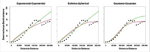
Figure 7 Experimental semi-variogram (dots) and fitted models (red line: ordinal least squares, green line: weighted least squares) for remotely sensed SST data from the Malpelo FFS. Distances are given in meters.
Table 4 Positions in geographic (GCS_WGS_1984) and planar coordinates (MAGNA Colombia West) of the stations of the sampling network for oceanographic sampling in the Malpelo FFS.
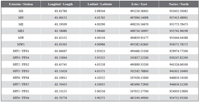
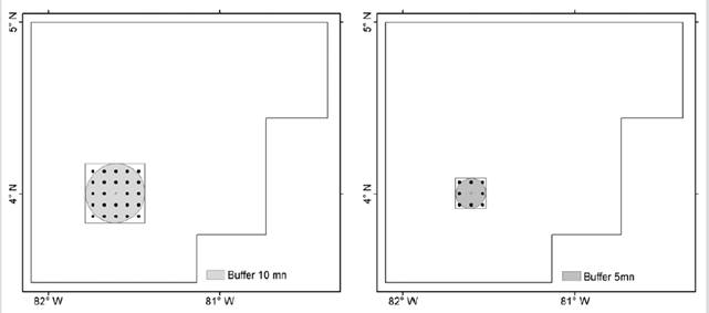
Figure 8 Sampling network for oceanographic monitoring of the Malpelo FFS, with a distance between stations of 7.41 km (4 nm) and for an area of influence of 18.52 km (10 nm) (left) and 9.26 km (5 nm) (right).
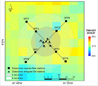
Figure 9 Sampling network proposed for the oceanographic monitoring of the Malpelo FFS, with a distance between stations of 7.41 km (4 nm) around Malpelo Island and taking into consideration the displacement axes of the currents. A Sea Surface Temperature (SST) image from the MODIS-Aqua sensor of July 2019 is superimposed.
DISCUSSION
The efforts of the Pacific Territorial Directorate (DTPA in spanish) of the National Natural Parks (NNP) to maintain monitoring of oceanographic conditions in the Malpelo FFS over time have been immense. Since the initiation of the process in 2006, the DTPA has had to overcome the logistical difficulties of sampling in a remote oceanic area and been obliged to make use of available platforms, such as dive ships. However, the surveys have been conducted on a sampling network with a small number of stations, separated by very short distances, with the result that the spatial variability captured by the network is limited. It is not known what criteria were used to arrange the stations in the current sampling network, but it has remained unchanged since the beginning. In terms of temporal variability, the coverage is also insufficient, due to the difficulty of maintaining continuous or monthly monitoring in this remote area. However, sampling has always been attempted in at least one of the months of the two contrasting seasons, namely between February and April, when the northern trade winds predominate and seasonal upwelling and SST decrease because of the winds of the Panama jet (Chelton et al., 2000) and between September-October, when the southern trade winds predominate and SST is higher than during the first half of the year.
The monitoring of biological or oceanographic conditions in marine or aquatic systems should allow for a unifying approach and capture as much variability as possible along different spatial and temporal scales. It should also ensure that the arrangement of stations is not redundant, as this unnecessarily increases costs. In the spatial arrangement of sampling stations, the most common approach to the design of a sampling network involves the use of quadrats and transects, according to the assumption that the samples are independent. However, a possibly more robust alternative is to assume that the phenomenon to be studied represents a stochastic process in which the measured variable is regionalized which allowsmaking it possible to study its spatial autocorrelation structure. In this regard, Giraldo et al. (2001) and Giraldo (2002) propose procedures that are based on criteria associated with the distance between pairs of points, such that a semivariogram can be calculated. This has been the approach used in this paper.
When fitting the semivariograms for the in situ SST data, the mean squares of the error were equal to zero. This is an indicator either that the distance between the in situ sampling stations is insufficient for there to be considerable SST variability or dissimilarity, or that there are too few stations. Therefore, from this data set it was not possible to construct a robust semivariogram model that would provide information useful for adjusting the sampling network in the Malpelo FFS. This reinforces the need to increase the number of stations in the oceanographic sampling network of the Malpelo FFS.
The range found in the best fit model (179,340 m for the analysis with remotely sensed SST data) is relatively high considering that the maximum distance between the southwestern and north-eastern ends of the sanctuary is 255.3 km (137.8 nm). In other words, in the Malpelo FFS two SST values are independent at 179.3 km (96.8 nm). At shorter distances the values will be spatially autocorrelated. According to Giraldo et al. (2001), this condition is ideal because the predictions obtained by geostatistical interpolations will have a lower variance and a lower prediction error, as found in the sampling network with stations every 7.41 km (4 nm). Therefore, a reduced number of sampling sites will be required and reduced confidence intervalsmight be obtained when the variable is estimated. In addition to the spatial variation examined with reference to semivariograms, the proposal for the new sampling network presented here -which includes the first two rings of the 7.41 km network - takes into account the dominant effects during the first quarter of the year of the cyclonic gyre associated with the effect of the Panama jet and the development, during the period of dominance of the southwest trade winds, of an anticyclonic gyre in the eastern sector of the PB and a cyclonic gyre in the western sector (Rodríguez-Rubio and Giraldo, 2011).
Since the proposed sampling network took logistical limitations into account and limited the number of stations to the first two rings of an ideal network of 598 stations, the proposal to monitor the oceanographic conditions of the Malpelo FFS may be modified to the extent that the sampling conditions might improve. If a vessel appropriate to the demands of the oceanic zone and dedicated exclusively to oceanographic monitoring were available, a third sampling ring could be added. It should be clear that in either case the area of coverage is still insufficient. Of the 2,709,612.8 ha that currently make up the sanctuary, the proposed expansion of the sampling network only covers 49,568 (1.83 % of the protected area). Therefore, in a sector such as the Malpelo FFS, whose vast marine area represents great logistical and economic challenges to maintaining continuous sampling over time using a network of stations that is sufficient to capture the variability of the processes involved, in situ monitoring should be complemented with remote sensing. This would make it possible to evaluate variability at different spatial and temporal scales and to guide management decisions more accurately.
CONCLUSIONS
The current sampling network used for the oceanographic monitoring of the Malpelo FFS, which has stations located at 0.93 km (0.5 nm) and 1.85 km (1 nm), from the island, presented reduced spatial variability, showing that during the period 2006-2019 the monitoring was conducted over a body of water with similar surface characteristics, allowing it to be assumed that the sampling was redundant. In addition to it covering a very small area, the semivariance models indicated that the same results could have been achieved with a smaller number of stations. Therefore, the proposal to expand the sampling network responds to the needs of the protected area, since the new sampling network will permit the capture of a greater variability of the processes associated with sea temperature. In this sense, the decision to propose a new sampling network was based on the dissimilarity between stations associated with the semivariance model, the variance of the prediction error, the predominant marine current pattern during the annual cycle and logistical aspects related to the limitations of the distances covered by the vessels that carry out oceanographic monitoring in the Malpelo FFS. The proposed sampling network has eight new stations. The possibility of maintaining the six historical stations is also considered, although this number could be reduced to only four, for a total of 12 stations.
According to the Management Plan of the protected area (Parques Nacionales Naturales, 2015), the oceanographic component is of great importance to ensuring understanding of the distribution and abundance of the protected area’s conservation assets and guiding management strategies. This is why it is important to maintain a continuous record of physical, chemical and biological variables in the area. This requires a specific work platform that can remain in the area long enough to carry out the required sampling, something that may not be possible due to logistical and economic restrictions. Therefore, given the challenge of monitoring oceanographic conditions in the Malpelo FFS associated with its size and its distance from the coast, remote sensing is a cost-effective alternative that allows continuous monitoring in space and time, and is an alternative tool that could be used to generate information complementary to occasional in situ sampling.

