


 English (pdf)
 Article in xml format
 Article references
 Send this article by e-mail
 Cited by SciELO
  Cited by Google
  Similars in
SciELO
Similars in
SciELO  Similars in Google
 Permalink
INTRODUCTION
One of the objectives of agriculture is to improve the yield of crops (Cortés et al. 2013). Consequently, tools for the analysis of soil variability must be available, given that soils have no homogeneous characteristics (Stadler et al. 2015) and traditional measurement processes make the analysis of crop variability inaccurate. Growing conditions in crops change depending on variables such as apparent electrical conductivity (ECa) and soil moisture. Therefore, this situation requires actions to estimate these parameters, which are directly associated with crop yield. This also seeks to obtain efficient land management to reduce the negative impact on the environment (Stadler et al. 2015).
Some of the tools that are used for the study of crop variability are information and communication technologies (ICT) to optimize the production of crops in such a way that makes it possible to modify soil management in a specific site (Corwin & Lesch, 2003). For the inclusion of these technologies in agriculture, it is necessary to identify the variables that allow obtaining a direct relationship with the properties of the soil, and there is evidence that ECa and soil moisture fulfill this role. On the one hand, soil moisture depends on several soil properties, such as porosity, degree of compaction, soil structure, organic content, and temperature, among others physical characteristics (Susha Lekshmi et al. 2014). ECa, on the other hand, is a variable with which different parameters of the soil can be associated, such as salts, nutrients, water content, productivity, and crop growth (Stadler et al. 2015).
The measurement of soil moisture can be done using widely known techniques, such as the reflectometry technique (Menziani et al. 1996), capacitive technique (Eller & Denoth, 1996), gamma ray technique, neutron scattering technique (Susha Lekshmi et al. 2014) and electric impedance technique. The most frequent methods for the measurement of soil moisture are dielectric techniques, which consist in finding the dielectric constant associated with the capacitance. The main differences between the existing methods are in the associated cost and the technology used. The ECa can be measured by obtaining electrical resistivity or electromagnetic induction (Corwin & Rhoades, 1984). Within the resistive technique, there is the 4-electrode resistivity method, which has two variations that are frequently used: The Schlumberger-Palmer arrangement and Wenner´s arrangement (Wenner, 1915).
It should also be noted that the use of ICT allows conducting of studies on the yield and feasibility of soils by mapping the data obtained in real-time and then, obtaining more detailed information about the soil under study (Rambauth Ibarra, 2022). Consequently, this article presents the analysis and development of two measurement devices for obtaining ECa and soil moisture with its geolocation and with the least failures. The system was implemented with software in python language on the Raspberry Pi 3 board, in to provide low-cost equipment for the soil analysis and allow increased access of small farmers to these technologies.
MATERIALS AND METHODS
Measurement methods
Method for calculating the soil ECa. Wenner’s method was used for the device configuration since the separation between electrodes is constant just as in commercial devices. Additionally, the electrode length does not change and therefore the measurement is not affected (IEEE, 2012). The pair of internal electrodes measure the electric potential difference (V) and the two external electrodes measure the electrical current (I). The resistance associated with a fraction of soil area is obtained using Ohm's law: R=V/I. Wenner's arrangement (Figure 1a) is characterized by equid-spaced electrodes at a uniform distance that allows obtaining the resistivity in a determined area of the ground, and the measurement depends exclusively on the internal electrodes of the array. Apparent resistivity (ρ) was calculated with equation 1 (Wenner, 1915).
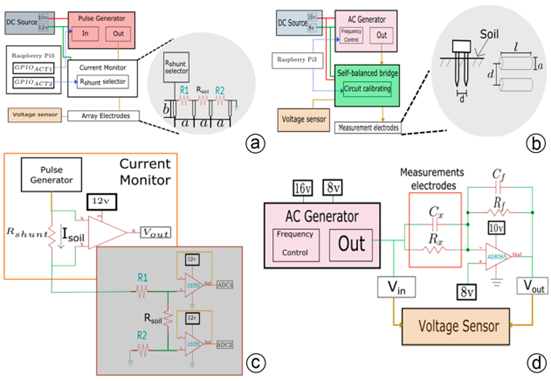
Figure 1 Methods of measurement for testing and hardware design for in situ tests. a) In the right, the Wenner’s method for measurement of soil resistivity with 4 electrodes. In the left, the complete system of measurement of the apparent electrical conductivity with Raspberry pi 3; b) In the right, the capacitor of parallel cables for measurement moisture soil. In the left, the complete system of measurement of the moisture soil with Raspberry pi 3; c) Final device for measurement of current of soil and electrodes voltage for ECa; d) Final device for measuring moisture soil with self-balanced bridge configuration.

Where a is the distance between electrodes and b is the electrode length. The ECa is computed with equation 2.

Method for calculating soil moisture. In this work, the electric impedance technique was chosen, due to the ease to obtain the variable of interest and the cost associated with the practical implementation of this method (Susha Lekshmi et al. 2014). To obtain soil moisture, the principle of dielectric permittivity was used and denoted as εr. This is a parameter associated with most fluids, including water, and allows obtaining fundamental characteristics. Therefore, to implement the electric impedance technique, an electronic configuration known as the self-balanced bridge is used as shown in figure 1d. Through this configuration, the capacitance of the fluid present in the soil was obtained, which is directly related to the electric impedance and its moisture. The estimation of water content θ of the soil was made by computing the value of εr, which is associated with the soil moisture percentage obtained by the ML2X commercial sensor (ICT International, 2015) in a total of 100 soil samples of the Marengo Agricultural Center (CAM) with different moisture content (mainly silt soil and clay soil with high content of sodium and salts). Likewise, this sensor was calibrated to be used as a standard in the measurement of soil moisture content. Once the values were obtained, the weighting was performed and the equation 2 with the best coefficient of determination for the volumetric water content was calculated.
Hardware design
ECa sensor. For the measurement of the electrical conductivity of soil, the system comprised a transmitter, a receiver, a power source, and electrodes connected to the ground (Seidel & Lange, 2007). It is necessary to use an AC generator, because using DC in the ground may produce spontaneous polarizations in the soil. To determine the appropriate values of the ECa sensor devices, tests were performed on soil samples with different values of water content (between dry and saturated soil). The test involved feeding the Wenner’s array electrodes with 60 different values of low-frequency voltage (between 0.1 Hz and 10 Hz) to avoid polarization between electrodes due to DC current (Seidel & Lange, 2007), and thus establish the appropriate minimum and maximum voltage values of the generated AC signal.
For this purpose, the DC current was injected through 4 electrodes, in this case, 4 stainless steel rods with an approximate diameter of 1/4” (Wenner, 1915). The distance between each pair of electrodes is a constant value, in the same way, the length of each rod is equal for the 4 of them (IEEE, 2012). The measurement of the current flowing through the electrodes was made through a current monitor circuit (Figure 1c). This electronic configuration comprises an operational amplifier and a bypass resistor, and the selected current monitor is the integrated circuit INA213 (Texas Instruments, 2017). The derivation resistance is connected to the integrated differential inputs, and it was selected using the estimation of values given with the soil samples of the CAM. Additionally, it was decided to set up a monitoring system (Figure 1a) to control the selection of the resistance connected to the differential terminals of the current sensor. The change of resistance was made through a digital control from the embedded system, by choosing the resistance according to the current values measured.
The measured potential difference was obtained from the internal electrodes of Wenner’s arrangement. To take this measure, the LT1055 op amp (Linear Technology, 1994) was used as a voltage follower. The differential variable of soil voltage was digitally obtained in the Raspberry Pi 3 board, by detecting the voltages in each of the internal electrodes of Wenner’s method (the voltage over Rsoil in Figure 1c).
Moisture sensor. The moisture sensor is composed of a circuit that generates a sine wave connected to the self-balanced bridge, a pair of electrodes inserted into the soil (Figure 1b), a circuit that allows calibrating the behavior of the self-balanced bridge, and a voltage detector circuit. The self-balanced bridge configuration comprises an operational amplifier AD8065 (Analog Devices, 2016), a transducer element formed by an analog peak detector to obtain the input and output voltages, an alternating current source made with the integrated circuit XR2206 (Exar Corporation, 2008), an unknown impedance (reactance given by the soil, measured with electrodes of the moisture sensor), a known impedance formed by a resistance (Rf) and a capacitor (Cf) in parallel of values 3kΩ and 223pF (Figure 1d). Starting from equation 3 the unknown capacitance is determined.

where CX is the unknown capacitance of soil, Cf is the known capacitance, Vinput is the input voltage and Voutput is the output voltage. With this value, the approximate value of the soil dielectric permittivity can be found by using equation 4.

Where Er is the dielectric permittivity, E0 is the dielectric permittivity in free space and Kg is the capacitor geometric constant.
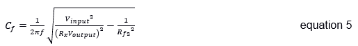
Additionally, to avoid voltage drops due to parasitic loads, a voltage follower with the AD812 operational amplifier (Analog Devices, 1998) was used between the signal generator circuit and the self-balanced bridge. Also, given the variable behavior of the capacitor at different frequencies, the circuit was evaluated in different ranges through a simulation analysis of the frequency response to determine the values of the known impedance of the self-balanced bridge, thus allowing a stable operation of the device (Agilent Technologies, 2006). Equation 5 was used to obtain the capacitance Cf of the circuit for the calibration.
The voltages Vinput and Voutput from equation 3 and equation 5 were obtained using an analog peak detector, which provides rapid detection and filters the signal avoiding noise. This peak detector was finally coupled to a voltage follower, with LT1055 amplifiers to avoid any voltage drop when connected to the Raspberry Pi 3 board. The measuring electrode design was based on a capacitor of parallel cables, using the following geometric considerations: stainless steel rods with a length (l) of 13 cm and diameter (a) of 3 mm (Figure 1b). All of the above was digitally controlled by the Raspberry Pi 3 board.
Embedded system and peripherals. The device required a data processing system; thus, the Raspberry Pi 3 board was used (Raspberry Pi Foundation, 2016), likewise, an integrated and compact user interface was programmed, using a 7" touch-sensitive screen to avoid the use of external peripherals, a tablet keyboard, and a small-sized frame to protect the device. The board works with a 5V to 2A power supply, since its current consumption increases if external peripherals are connected. To obtain the GPS measurements, a UBLOX NEO 6M module was used, which can be connected through one of the USB ports of the Raspberry Pi 3. Since the board needs an external A/D converter, the integrated ADS1115 was chosen, as it provides a 12-bit precision and different gain options to obtain measurements in the millivolt range (mV).
Software design. The values of interest (ECa and soil moisture) are determined by two equations from the designed program, through the digital voltages collection associated with each sensor. Another programmed function is to obtain the geographical location (GPS) of the measurement with its associated parameters (ECa and moisture), which are reported in an Excel file. The programming was made in Python language.
In situ testing. The measurements were made at the UNAL campus located in the city of Bogotá, D.C. at the geographical coordinates 4°38'N, 74°04'O and at the CAM located in the municipality of Mosquera, Cundinamarca, at the geographical coordinates 4°42'N, 74°12'O. In the first case, 18 measurement points were determined randomly around the campus, using a 10 cm length ECa sensor electrode and the moisture electrode. Three different measurements of each variable were taken at each point to determine the data repeatability in the different measurements of the same point between 9:00 am and 12:00 pm. For these tests, the weather conditions were affected by constant rain and relatively high humidity in the environment, which allowed testing of the prototype in extreme conditions.
For identifying the viability and efficiency of the sensors’ final design, the CAM was chosen for in situ testing in four soil lots the same day, in the time slot between 8:00 am and 4:00 pm. A total of 60 testing points aleatory distributed in the lots were obtained. The measurements were randomly distributed as follows: 13 measurements in Lot 3, 16 measurements in Lot 7, 14 measurements in Lot 12, 14 measurements in Lot 13, and 3 measurements on the way between Lot 7 and Lot 3, for a total of 60 samples obtained. With the previous planning in the measurement distribution, a single intake per point of both ECa and moisture was performed. Multiple measurements per point are not required, given the existing repeatability. The soil lots chosen on this date have no crops in their surfaces, are principally pastoring zones, and the grass specie is fundamentally kikuyu (Pennisetum clandestinum). The weather conditions for this day were the following: cloudy sky, absence of rain, temperature of 21 ºC approx., and relative humidity of 50 to 73 %.
Feasibility study of the design. This analysis was made through the estimation of the costs of the final prototype, which was compared with some commercial devices to establish its relevance for small farmers.
RESULTS AND DISCUSSION
First, a set of tests were established with soil samples in different conditions of water content to determine the requirements for the design of the sensors. In the second stage, a validation test from the functional designs was made with a soil sample equally controlled in the laboratory. Third, the evaluation in situ was concluded for evidencing the operability of the proposed designs and, finally, to identify the economic feasibility of the designs.
Sensor design
ECa sensor. The range of voltages contained between 1 and 30V (Figure 2a) shows the experiments in different voltage levels, thus allowing finding the approximate values of soil resistance. Figure 2a shows only two cases of the study, dry and saturated soil. Likewise, the current levels flowing over the selected samples were detected, thus finding the appropriate derivation resistance values for the current monitor circuit. The assembly diagram resulting from the electronic configuration is shown in figure 1c. Table 1 details the approximate current values measured in cases shown in figure 2a. The current monitor derivation resistance (Rshunt) selection was established with the values found by the numerical calculation with Ohm’s law which was 5.6 and 220Ω, thus allowing optimal operation in soil measurements. Finally, the design of the measurement electrodes was specified according to the considerations established by Wenner’s arrangement in terms of length and depth (IEEE, 2012). Three dimensions were manufactured with a length of 25, 20, and 10 cm, and the separations between electrodes were established according to their length and depth as follows: 4, 3, and 2 cm, respectively. With the dimensions, the geometric constant of Wenner’s arrangement was calculated and included directly in equation 1 through the software implemented.
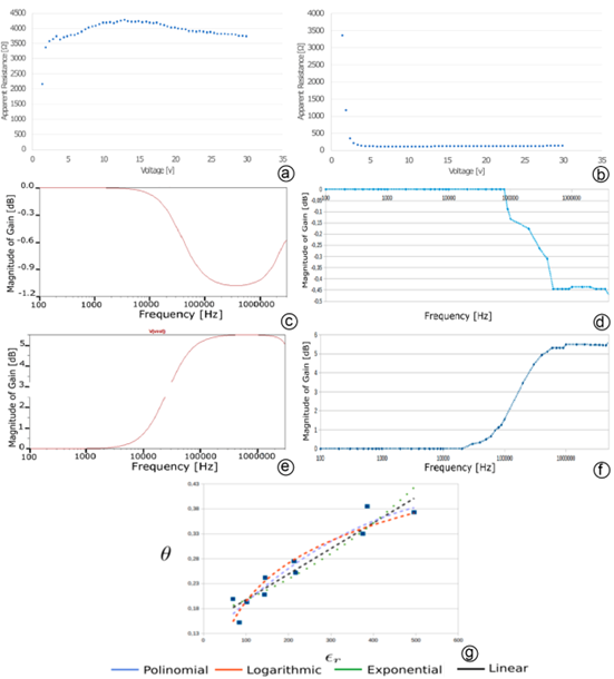
Figure 2 Testing for controlled samples in laboratory for sensor calibrating and final device selection. Testing for measurement apparent resistance: a) dry soil; b) saturated soil. Test for estimating the most stable range of frequencies in dry soil: c) bode diagram in simulation; d) real values on self-bridge balanced. Test for estimating the most stable range of frequencies in saturate soil: e) bode diagram in simulation; f) real values on self-bridge balanced; g) Ratio between dielectric permittivity ( ε r ) and moisture content of soil (𝜃) for estimating the associated equation with better 𝑅 2 coefficient.
Table 1 Current values in saturated and dry soil for the controlled samples in the laboratory.
*The measurements were realized with commercial AC generator and DC source. The values of voltage and current were obtained with Fluke multimeter and commercial oscilloscope Tektronix.
Moisture sensor. To establish the moisture sensor final design, an initial measurement was made of the capacitance value given by the soil samples in a range value between dry and saturated conditions, resulting in the following values: 29pF-picoFarads- (dry soil) and 275pF (saturated soil). This data allowed us to infer that the values of capacitance in the soil are too low, so to obtain more efficient measurements and with low errors, high frequencies should be used (Susha Lekshmi et al. 2014). Additionally, to determine the circuit behavior in different frequency ranges and, consequently, to stabilize its behavior for the desired frequencies, the assembly shown in figure 1d was implemented using two values of unknown capacitance instead of the actual measurement electrodes (simulating the soil behavior) and in agreement with the previously obtained values of soil capacitance in a dry and saturated condition. The circuit behavior for the two capacitance values Cx was verified, by performing a sweep of frequencies between 0 Hz and 3 MHz with each capacitor. The practical results were compared with those expected in the simulation, as shown in figure 2b and 2c (Bode diagrams). In figure 2b it was shown that the behavior of soil is purely resistive below 100 kHz, on the other hand, figure 2c showed that at frequencies above 100 kHz, the gain of the self-balanced bridge depends exclusively on the relationship given by equation 2, and soil has a capacitive behavior. Therefore, these plots allowed to determine the circuit stability implemented in the range between 500 and 2 MHz. These sets of frequencies were taken as the measurement interval for the final device to obtain soil moisture in the in-situ test.
Additionally, a circuit for calibrating the self-balanced bridge was also established, due to possible fluctuations in the value of the known capacitor Cf, which generates changes in the system. Finally, the self-balanced bridge circuit was implemented with the calibration resistors of 120 Ω (alternate value of Rx) and 220 Ω (alternate value of Rf), and the values of the known capacitance Cf. The laboratory test showed that the change in frequency directly affects the value of the capacitor and that it is important to perform a constant calibration of this capacitance, since the numerical calculation of the soil capacitance, according to equation 2, is proportional to the value of the capacitance that must be calibrated.
With the design of the finished device, tests were made in the laboratory-controlled soil, performing various measurements with 10 soil conditions of moisture contents. To avoid bad measurements, the samples were irrigated with water without chlorine. The testing consisted in taking 10 measurements of each moisture state in the frequency range of interest. The water content value θ was obtained with the commercial sensor, and the dielectric permittivity was calculated using equations 2 and 4. These results allowed establishing that the variation in the value of dielectric permittivity is lower in the range of frequencies from 1.4MHz to 2MHz, with a value of Er = 106.2 in 1.5MHz and a value of Er = 90 in 2MHz. The values of dielectric permittivity are higher and more unstable in low frequencies.
Then, the equation associated with the soil water content was determined by relating the data average per dielectric permittivity obtained in the different soil moisture conditions with the estimation of the commercial sensor of the water content. Likewise, the data obtained were associated with 4 trend lines, as shown in figure 2d. The associated equations for trend lines for the dispersion graph were:
Linear. θ = 0.513×10⁻³ εr + 0.146. R2=0.907.
Polynomial. θ = -6.69×10⁻⁷ εr 2+0.87×10⁻³ εr+0.111. R2=0.9257 .
Logarithmic. θ = -0.1109lnεr -0.3167. R2=0.8946.
Exponential. θ = 0.1629e1.92×10^-3 εr R2=0.8602 .
Consequently, the line with the best coefficient of determination is the one belonging to the second-degree polynomial function, which has an R2 = 0.9257. Finally, the separation between the electrodes of the moisture sensor was established, taking into consideration the geometric constant of a parallel cable capacitor (Eller & Denoth, 1996). By taking the 13 cm length (l) and the 3 mm diameter (a), it was found that the minimum spacing between rods is 3 mm, so it was decided to choose a separation (d) greater than 1.5 cm (Figure 1b), to achieve a geometry factor of Fg = 0.1782 and avoid design problems and implementation by a minimum separation.
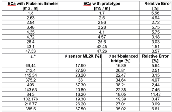
ECa sensor evaluation results. The sensor evaluation tests were performed in laboratory-controlled samples with two FLUKE multimeters. The voltage and current measurements were taken on Wenner’s array electrodes. Likewise, the same measurements were made with the proposed prototype, and some of the results are shown in table 2 (only dry and saturated soil conditions). The relative error is under 6 % in controlled conditions, with ambient temperature and relative humidity of 45 % in the environment. The measurements were made with many soil samples and different soil moisture conditions (between dry and saturated soil). A total of 30 measurements were taken for each soil moisture condition in the range of 1 and 30V values. ECa was estimated for a total of 10 moisture conditions. These results were consistent with the behavior expected of soil, which is moderately and highly saline.
Table 2 Results of evaluation of the final prototype for measurement of ECa and moisture of soil with relative error.
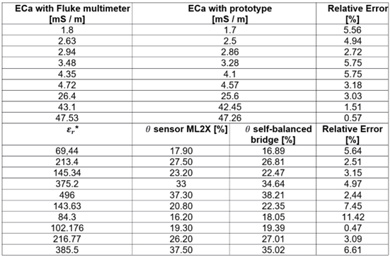
*The dielectric permittivity is dimensionless. 𝜃 value refers to water content that its directly related with moisture content of soil.
Evaluation results of the moisture sensor. The proposed moisture sensor was checked by performing measurements on soil samples with different moisture contents. A total of 100 measurements were averaged in a total of 10 soil moisture conditions for determining its dielectric permittivity. Moisture percentages identified were between 15.2 and 38.5 % (Table 2), without a specific order to avoid altering the measurements. Table 2 establishes the error in the actual measurements of the percentage of soil moisture (only some measurements). As demonstrated, the variations of the values measured with the self-balanced bridge and the commercial sensor are below 7 % (except for one measurement). This gives a percentage of reliability suitable for the prototype, very close to commercial devices.
The final prototype included the designs obtained with the previous analyses from each sensor in two PCB designed for this purpose, whose final implementation can be observed in figure 3a. The portable frame for the protection of the whole system is shown in figure 3b, including the peripherals used (GPS, electrodes for measurement, 7” screen, keyboard).
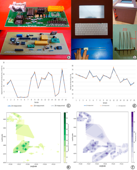
Figure 3 Final device and in-situ testing: a) final circuits on PCB. Up, the circuit of CEa sensor and down, the circuit of moisture sensor; b) Final prototype. Up, the box with screen and keyboard, with the circuits and peripherals necessary for its operation. Down, the electrodes for moisture and CEa measurements. Dispersion measure from the data obtained in UNAL Campus: c) CEa data; d) moisture data. Mapping with data from CAM obtained in the 4 lots: e) CEa data; f) moisture data.
In situ measurements in the UNAL Campus and CAM. From this experiment, it was determined that the obtained values did not fluctuate and were constant, thus they were used to make the respective scatter plots observed in figure 3c. Once the previous measurements were completed, it was concluded that the data obtained yielded precise information that fits the stability considerations found in the laboratory tests.
Finally, in the CAM, 60 measurements were taken in the 4 selected lots. With this consideration, random points were established without a constant pattern per lot, so that there was no relationship between distributions of points in the selected lots. As indicated before, one of the project objectives is to obtain real-time data mapping that facilitates visualization in the field. This is evidenced in the contour plots obtained through the software developed, and in real-time in the prototype represented in figure 3d. The measurements obtained have coincided with the soil characteristics of the CAM lots, so high reliability of the measurements in the designed devices is reported.
Economics feasibility of the final design. In the study of the feasibility, the comparison of average prices of principal commercial manufacturers (Delta T, Decagon, Omega) was included for sensors and portable sensor kit. With the final price, the prototype was developed. The total associated cost to the final device for this work is approximately the fourth part of the average price of the basic portable sensor kit for the measurement of both variables (approximately US250 at present). Consequently, this design involved choosing between different alternatives for ECa measurement and soil moisture. By implementing those with the highest cost-effectiveness ratio, it was demonstrated that the system has low cost, and is an alternative for small farmers accessing these technologies and achieving better yield in the crops. As an important result, the integration of an embedded system with sensors for agricultural use, together with the use of geolocation, enhances the use of these technologies for their implementation in on-site measurements, thus establishing the importance of ICT for soil study. As an added value, this device has the capacity of making graphs in real time of the measured variables in soil and storing the historical data in excel archives.
Finally, it should be noted that the greatest contribution achieved in this project, regarding the agricultural sector, is to provide a functional design, low cost, and with good precision for the chosen variables of soil diagnosis (ECa and Moisture). It is expected that these designs will serve as a basis for further studies in this area, which could add improvements for greater reliability in the data, including characteristics from different types of soils.
In this work, the design of a system that allows the estimation of the ECa and the moisture of soil was reported. The realization of this design involved choosing between different alternatives for ECa measurement and soil moisture, to implement those with the highest cost-effectiveness ratio.
As an important result, it is shown that the integration of an embedded system with sensors for agricultural use, together with the use of geolocation, enhances the use of these for their implementation of on-site measurements, establishing the importance of the ITC for soil study.
It should be noted that the greatest contribution achieved in this project, as regards the agricultural sector, is to provide a functional design, low cost, and with good precision for the variables of soil diagnosis chosen (ECa and Moisture). It is expected that these designs will serve as a basis for further studies in this area, which could add improvements to have greater reliability in the data, including characteristics from different types of soils.

