


 English (pdf)
 Article in xml format
 Article references
 Send this article by e-mail
 Cited by SciELO
  Cited by Google
  Similars in
SciELO
Similars in
SciELO  Similars in Google
 Permalink
INTRODUCTION
Mobile robots differ substantially from traditional manipulators due to their ability to move autonomously in a dynamic environment. The dynamics of these robots, as described in Muir and Neuman (1987), are influenced by the configuration of their wheels, which affects their interaction with space and, consequently, their movement. This interaction is fundamental in the navigation of autonomous vehicles, as indicated by recent studies (Juárez-Lora & Rodríguez-Ángeles, 2023; Meng et al., 2018; Paden et al., 2016; Zhang et al., 2021).
The path following problem has been widely studied in the literature, with various control algorithms proposed to address this task (Rubio et al., 2019). However, the inclusion of noise in the simulation of these algorithms is less frequent, despite being a critical factor in real-world applications. This work seeks to fill this gap by providing a comprehensive comparative evaluation of popular control algorithms in the presence of noise.
Four control strategies were selected for this study due to their relevance and extensive use in the literature: proportional-integral control (PIC), feedback linearization (FL), Lyapunov-based control (LBC), and model predictive control (MPC). Proportional control is one of the simplest and most widely used controllers in industrial applications. Its inclusion serves as a basic reference for comparison (Maxim et al., 2019; Meng et al., 2018). FL transforms nonlinear systems into linear ones, facilitating their control, which is especially useful in mobile systems with a prevalence of nonlinearities (Bascetta et al., 2022). LBC offers stability guarantees for nonlinear systems, which is crucial in environments with disturbances (Uddin, 2017), and, finally, MPC is known for its flexibility and ability to handle explicit constraints. It has proven to be effective in various robotics applications (Guo et al., 2019; Chaib et al., 2004).
One of the main challenges in comparing controllers is ensuring a fair and equitable evaluation. The selected controllers operate under different principles and designs, which means that the inclusion of the same noise source for all does not always ensure a fair comparison. It is essential to identify the exact point where noise affects the system, be it at the input, the controller output, or the actuator. In this study, four types of noise are used: Gaussian, uniform, impulsive, and colored (Lu et al., 2021). Including the same noise source for all controllers does not guarantee that performance will be affected by the controller itself - it could be affected solely by the noise source.
Mobile robot control includes multiple approaches and techniques, from classical controllers to modern methods such as adaptive and robust control. Despite the wealth of available methods, the simulation of these controllers under noise conditions remains a little explored research area. Previous studies have addressed the use of proportional-integral, proportional-integral-derivative (PID), and model predictive controllers in mobile robots (Bakker et al., 2010; Özdemir & Öztürk, 2017), as well as techniques based on Lyapunov theory and sliding mode control (Zhai & Song, 2019; Wang et al., 2019). However, few studies have systematically evaluated the impact of noise on these algorithms. This work aims to fill this gap by including random noise in simulations and detailed numerical evaluations, providing a significant contribution to the existing literature.
The main objectives of this study are to evaluate and compare the performance of different control algorithms in mobile robots under noise conditions, identify the strengths and weaknesses of each algorithm in terms of robustness and stability, and provide recommendations on the selection of controllers for practical applications in mobile robotics.
This document is structured as follows. The next section describes the model of the differential mobile robot and the implemented control algorithms. Afterwards, the simulation results under both ideal and noise conditions are presented, and the final section discusses the results obtained and presents the conclusions of this study.
MOBILE ROBOT MODEL AND CONTROL ALGORITHMS
Differential mobile robot model
The kinematic model of a differential mobile robot is described by a set of equations representing its motion dynamics. As shown in Figure 1, the robot is equipped with two independently controlled driving wheels. The velocities of the left and right wheels are denoted as and , respectively, with r representing the wheel radius and L the distance between the driving wheel axes.
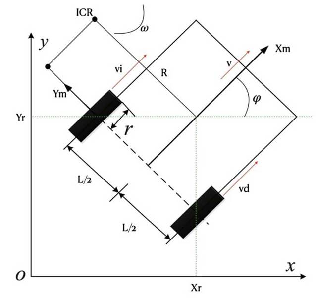
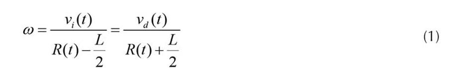
The robot's movement is based on the rotation of the wheels around their own axes and an intersection point called the instantaneous center of rotation (ICR). The angular velocity around this point is described by Equation (1).
The motion equations in the local reference frame are expressed in Equation (2).

The global reference frame is provided by Equation (3).

Implemented control algorithms
In this study, four widely used control strategies in the literature were implemented and compared:
Proportional-integral control. PIC is a classic and robust technique widely used in industrial applications due to its simplicity and effectiveness. Its goal is to minimize the error between desired and actual trajectories through proportional and integral adjustments. The PIC equation is presented in (4).

where KP and Ki are the proportional and integral gains, respectively.
Feedback linearization. This technique transforms nonlinear systems into linear ones, facilitating their control. It is especially useful in mobile systems where nonlinearities are prevalent. The transformation is achieved through a series of derivatives and the use of the system's Jacobian matrix. The general equation is presented in (5).

where F is the transformation matrix, and is the linearized input vector.
Lyapunov-based control. This method ensures system stability by defining a Lyapunov candidate function. The candidate function is selected such that its derivative is negative, ensuring the system's convergence to the equilibrium point. The control law is derived as follows:

where V(e) is the Lyapunov function, e is the error vector, and P is a positive-definite matrix.
Model predictive control. MPC is an advanced technique that optimizes system performance by predicting its future behavior and adjusting the control inputs accordingly. This type of controller explicitly handles system constraints and is defined through an objective function that minimizes the tracking error. This objective function is expressed in Equation (7).
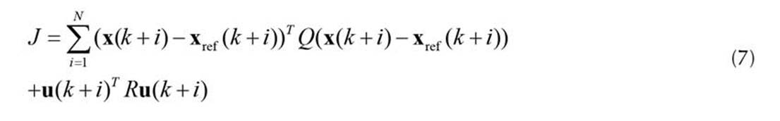
where Q and R are weighting matrices, x is the state vector, and u is the control vector.
Noise evaluation in the system
To evaluate the robustness of the control algorithms under noise conditions, four types of noise were considered:
Gaussian noise is characterized by a normal distribution, and it is used to simulate common random disturbances.
Uniform noise is equally distributed within a specified range and is used to evaluate the system's response to constant perturbations.
Impulsive noise consists of randomly distributed high-amplitude peaks simulating abrupt failures in the system.
Colored noise has a specific spectral distribution, and it is commonly used to simulate more complex environmental and process noises.
These noises were applied at different points in the system, including the input, the controller output, and the actuator, in order to accurately identify their impact on system performance.
Implementation and simulation
Simulations were carried out using the MATLAB simulation environment. Each controller was implemented and evaluated under both ideal conditions and each type of noise. The results were analyzed in terms of stability, accuracy, and robustness, using standard metrics such as the integral absolute error (IAE) and the mean squared error (MSE).
Integral absolute error
The performance of each control algorithm was measured using the IAE metric, which is defined in Equation (8).

where e(t) is the tracking error at time t, and T is the total simulation time. This metric was chosen for several reasons:
Simplicity and intuitiveness. The IAE is straightforward to compute and understand, making it an accessible metric for evaluating control performance.
Sensitivity to error size. By integrating the absolute value of the error over time, the IAE provides a comprehensive measure of the control system's accuracy, highlighting both small and large errors.
Relevance to industrial applications. The IAE is widely used in industrial control applications, providing a standard benchmark for comparing different control strategies.
Mean squared error
The MSE metric, as defined in Equation , was also used to evaluate the performance of the control algorithms.

where e(t) is the tracking error at time t, and T is the total simulation time. The MSE metric was chosen for the following reasons:
Error sensitivity. The MSE penalizes larger errors more than smaller ones, providing a clear measure of performance in contexts where large deviations are critical.
Common usage. The MSE is a widely used metric in control system performance evaluation, which facilitates comparisons with existing literature.
Variability insight. By squaring the error, the MSE provides insight into the variability of the error over time, complementing the IAE metric.
SIMULATION RESULTS AND ANALYSIS
This section presents the results of the simulations conducted to evaluate the performance of the four selected control algorithms (PIC, FL, LBC, and MPC) under various noise conditions. As previously mentioned, the impact of Gaussian, uniform, impulsive, and colored noise on the system's tracking performance was analyzed using the IAE and the MSE metrics.
To provide a consistent and challenging test for the control algorithms, a circular trajectory was selected for the simulations. Circular trajectories are commonly used in control system testing because they require continuous and smooth changes in both direction and velocity, thus providing a comprehensive assessment of the controller's ability to handle dynamic motion and maintain stability. This choice ensures that the controllers are tested under conditions that closely mimic real-world applications, where precise path following is critical.
Results for PIC
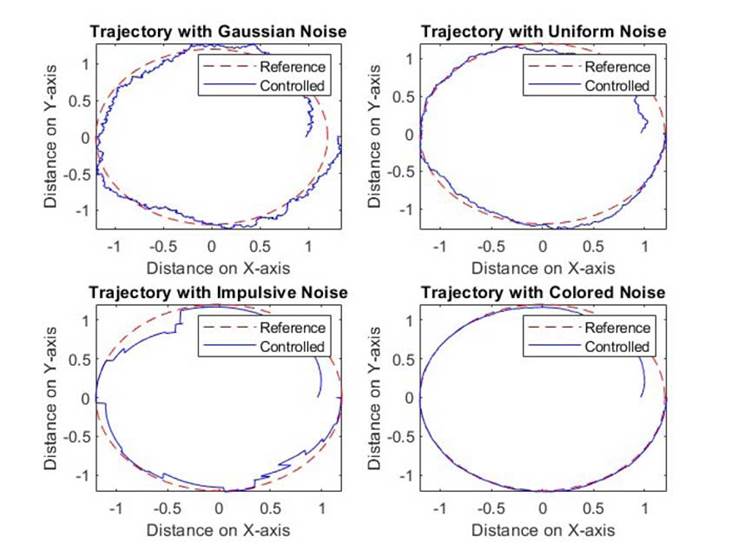
The PIC’s performance under different noise conditions is shown in Figure 2. The reference trajectory is depicted in red dashed lines, while the controlled trajectory is shown in blue solid lines.
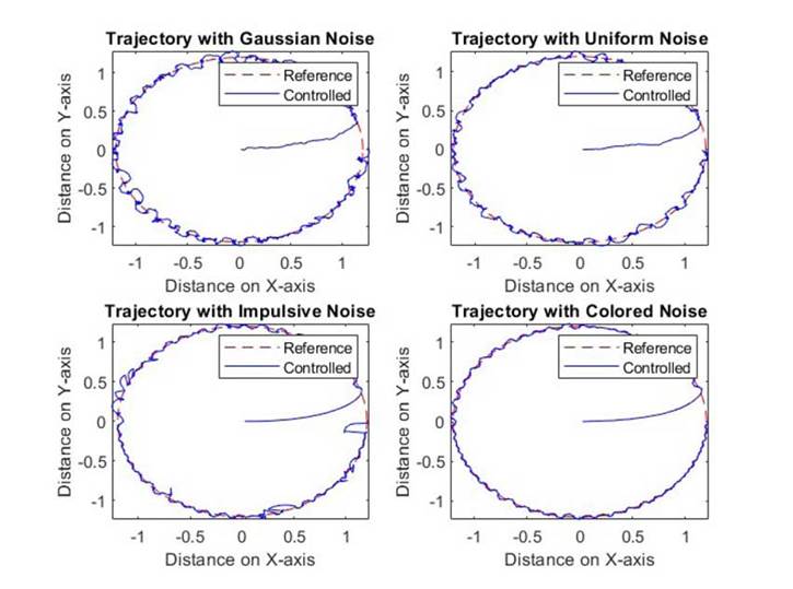
According to the results, the following can be stated:
Gaussian noise: The PI controller exhibits significant deviation from the reference trajectory, indicating sensitivity to random disturbances.
Uniform noise: The system shows moderate deviation but maintains a closer alignment to the reference compared to Gaussian noise.
Impulsive noise: Large deviations occur, demonstrating PIC's vulnerability to sudden, high-amplitude disturbances.
Colored noise: The performance is slightly better than that under Gaussian and impulsive noise but still shows considerable deviation from the reference.
Results for FL
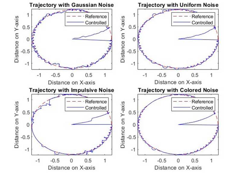
The performance of the FL controller is illustrated in Figure 3.
The results show the following:
Gaussian noise: This controller exhibits improved performance with respect to the PIC, with less deviation from the reference trajectory.
Uniform noise: The controller maintains a trajectory closer to the reference, indicating better handling of constant perturbations.
Impulsive noise: Despite the improvements, significant deviations are still observed, as the controller is susceptible to abrupt disturbances.
Colored noise: The controller performs well, closely following the reference trajectory in comparison with other noise types.
Results for LBC
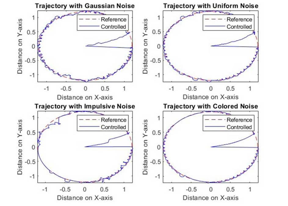
Figure 4 presents the results for the LBC.
In the above-presented graphs, the following can be observed:
Gaussian noise: The controller exhibits minimal deviation, demonstrating robustness against random disturbances.
Uniform noise: The controller shows an excellent performance, closely following the reference trajectory.
Impulsive noise: The controller maintains a better control, with smaller deviations when compared to PIC and FL control.
Colored noise: The controller performs well, indicating strong robustness to various noise conditions.
Results for MPC
The performance of the MPC is shown in Figure 5.
Gaussian noise: The controller exhibits good performance, with small deviations from the reference trajectory.
Uniform noise: The controller maintains a close trajectory to the reference, demonstrating effective handling of constant noise.
Impulsive noise: The controller can handle abrupt disturbances better than PIC and FL control.
Colored noise: The controller exhibits a good performance, maintaining a close trajectory to the reference.
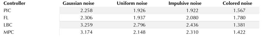
Comparative analysis using the IAE and the MSE
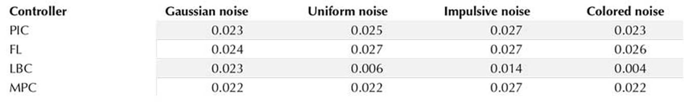
The IAE and MSE metrics were used to quantify the performance of each controller under the different noise conditions. The IAE values for each controller and noise type are summarized in Table 1, while the MSE values are presented in Table 2.
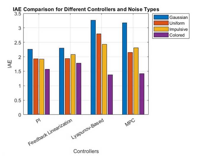
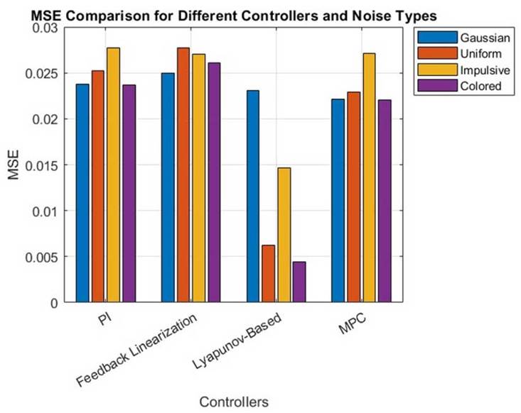
The bar charts in Figures 6 and 7 provide a visual comparison of the IAE and MSE values for each controller under the different noise conditions.
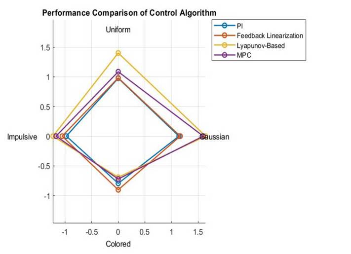
To facilitate the interpretation and comparison of the control algorithms’ performance under different noise conditions, Figure 8 presents a radar chart. This chart displays the integrated performance metrics for each algorithm across the evaluated noise types. Each vertex of the diagram represents a noise type, and the radar areas indicate the aggregate performance of each controller. A smaller spread in the diagram represents a better algorithm performance under the assessed noise conditions. This visualization synthesizes the results, clearly identifying the most robust algorithms based on their ability to minimize IAE and MSE metrics, and it provides an intuitive perspective on the controllers best suited for practical applications in noisy environments.
DISCUSSION
The results indicate that LBC and MPC generally outperform PIC and FL control in maintaining trajectory accuracy under noise conditions. Both LBC and MPC exhibit strong robustness, particularly under impulsive and colored noise, with minimal deviations from the desired trajectory. This behavior aligns well with their theoretical underpinnings: LBC ensures stability in nonlinear systems, while MPC effectively manages explicit constraints, making it ideal for handling disturbances.
The performance metrics reflect each algorithm's robustness and stability, showing their capacity to minimize trajectory deviations. Specifically, a lower IAE indicates superior accuracy in tracking the desired trajectory despite noise, while MSE provides additional insights into error variability over time. Controllers with lower IAE and MSE values show a better fit under high-noise conditions, highlighting the suitability of LBC and MPC for practical applications in mobile robotics, where robust and reliable control is crucial.
For a more detailed interpretation, the stability, precision, and robustness of each controller under various noise types were analyzed:
Stability.The stability of each controller was evaluated based on its consistent performance under different noise types. Specifically, the LBC, MPC, PIC, and FL display varied performance. LBC and MPC stand out with lower variability in both the IAE and MSE metrics, which is essential for predictable control in dynamic environments.
Precision.Precision, represented by a low IAE value in each controller, reflects these algorithms' ability to adhere to the desired trajectory. This is crucial in applications where precise movement control is required. MPC and LBC excel in minimizing trajectory-following errors under noisy conditions, while PIC and FL exhibit more notable deviations.
Robustness.The robustness of the LBC and MPC controllers is evident in their ability to maintain minimal deviations under strong perturbations, such as impulsive and colored noise. In contrast, PIC and FL showed vulnerability to high-magnitude disturbances. LBC and MPC's capacity to operate in high-uncertainty conditions positions them as the most suitable choices for dynamic and noisy environments.
In summary, this analysis confirms that LBC and MPC, along with PIC and FL, play specific roles in the operation of autonomous mobile systems under non-ideal conditions. However, the results demonstrate that controllers achieving lower deviations in the face of disturbances -particularly LBC and MPC- are the most effective for applications in autonomous mobile robotics, where noise resilience is a critical factor.
CONCLUSIONS AND FUTURE WORK
In conclusion, this study highlights the importance of robust control strategies for mobile robots operating in noisy environments. The results indicate that Lyapunov-based and model predictive controllers offer superior performance, making them suitable candidates for deployment in real-world applications. Future research should focus on further optimizing these controllers, testing them in diverse scenarios, and exploring new hybrid and adaptive approaches to enhance their capabilities.
This study provides valuable insights into the performance of various control algorithms, identifying several areas for future research. These include extended real-world testing to validate the simulation results and assess the controllers' performance in practical scenarios, enhanced control strategies combining different algorithms for improved robustness and accuracy, the optimization of control parameters using advanced techniques, a comparative analysis with additional metrics such as settling and rise times, and the evaluation of the algorithms' robustness to system uncertainties. Additionally, adaptive and learning-based control methods should be explored to dynamically adjust to changing noise conditions and system dynamics while maintaining performance despite changes in the robot's dynamics or environmental conditions

