


 English (pdf)
 Article in xml format
 Article references
 Send this article by e-mail
 Cited by SciELO
  Cited by Google
  Similars in
SciELO
Similars in
SciELO  Similars in Google
 Permalink
Introduction
According to FAO [1], moorlands are fragile ecosystems of global significance because they host rich biodiversity and, most importantly, because they are sources of fresh water. Espeletia (Espeletia sp.) is one of the most representative species of moorland vegetation and is of great ecological value for the local ecosystem and for the water cycle [2]. In recent years, populations of Espeletia have been affected by climate change [3], allowing phytopathogen organisms to cause biotic stress in this species. Biotic stress is caused by the presence of microorganisms that affect the vegetable and reproductive structures of the host plant, leading to significant losses in terms of population. A reduction in the population of Espeletia is certainly undesirable since it is an essential type of vegetation in the moorland ecosystem [4].
As for the stress, the images have been used for its identification, as in the work of Susi'c, et al. [5] and Zibrat et al. [6]: where support vector machine classification, biotic and abiotic drought stress in tomato plants can be differentiated by combining hyperspectral imaging and partial least squares.
The use of unmanned aerial vehicles (UAV) has become more frequent in recent years due to their multiple applications in fields such as cartography, photogrammetry, topography, precision agriculture and environmental monitoring, among others [7], [8]. Specifically, in the fields of precision agriculture and environmental monitoring, UAV have become commonplace since they allow images to be taken on a very frequent basis, which permits the identification of areas, either over fields or native vegetation, that require pest or weed control or any other type of intervention [9].
Regarding image processing, texture measurements have appeared in the literature since 1979, when the work of Haralick described texture as an important feature for the identification of objects or regions of interest in different types of images [10]. Based on the implementation of UAV platforms for remote sensing, a variety of applications are expected to make use of existing processing techniques, such as texture analysis [11]-[13]. Texture features have been used to process images captured by UAV platforms for different purposes. For example, in Laliberte and Rango [11] a study about herb identification in New Mexico, 10 types of texture identification measurements were used based on gray-level co-occurrence matrix statistics (GLCM) as well as gray-level difference vector statistics (GLDV). It was concluded that the incorporation of texture measurements significantly increases classification accuracy [11]. Likewise, to identify weed within fields of corn, beans and eggplants, texture analysis allowed a 17% increase in classification accuracy [9]. Even more, Feng et al. [13] used UAV images for urban vegetation mapping using random forest and texture analysis. Six least correlated GLCM texture features were calculated with nine different moving windows chosen in this study (3x3, 5x5, 7x7, 9x9, 11x11, 15x15, 21x21, 31x31 and 51x51). Results showed that overall accuracy increased from 73.5% to 90.6% and 76.6% to 86.2% after the inclusion of texture features, which indicated that texture plays a significant role in improving classification accuracy. Also, texture analysis has allowed the identification of hydric stress in Sunagoke moss [14] based on spectral analysis and GLCM texture features. Similarly, Hashim [15], [28] investigated the application of a backscattering imaging system (BIS) with different approaches of transform-based image texture analysis for the evaluation of banana quality at different ripening stages with Wavelet, Gabor and Tamura transforms. This study indicated that a BIS with transform-based image texture analysis coupled with computational intelligence techniques can be used for the evaluation of the quality of bananas. In the same way, Ferreira et al. [16] concluded that texture analysis of the panchromatic band enabled the detection of species-specific differences in crown structure, which improved tree species detection in tropical forests using World-View-3 images. Equally, the results [17] showed that combining the textural and spectral information during modelling resulted in improved classification of the sixteen green tea products compared to models built using spectral or textural information alone. More recently, in 2019, Yue et al. [12] estimated winter-wheat above-ground biomass (AGB) based on UAV ultra-high ground-resolution image textures and vegetation indices. They used eight gray-tone spatial-dependence matrix-based image textures to evaluate their correlation with AGB. These eight textures were typically based on the gray-tone spatial-dependence matrix defined by the Haralick. When calculating image textures, they have chosen three calculation windows: 3x3, 5x5, and 9x9. As a result, they concluded that the combined use of image textures and original visible images can help improve estimates of AGB under conditions of high canopy coverage.
This work focuses on texture analysis for images captured using UAV technology to identify the biotic stress of moorland Espeletia. Six different texture measurements from two main categories of texture analysis -statistical (first and second order) and model-transform approaches- are considered in this research work to compare their performance on the problem of differentiation of the biotic stress in Espeletia. Then, two different classifiers are applied, parametric and non-parametric approaches, to extract unhealthy Espeletia plants.
The paper is organized as follows. Some basic concepts are reviewed in Section 1. The general context that justifies the proposed method is presented in Section 2. The results obtained and its discussion are given in Section 3. Finally, conclusions are drawn in Section 4.
1. Basic concepts
1.1 Biotic stress
Stress is an external factor that negatively affects an organism or forces it to change the physiology of the plant. The factors that produce stress can be classified as abiotic stress or biotic stress [20].
Abiotic stress can be classified as physical and chemical, depending on the causative factor. Physical factors include stress due to water deficit or excess, extreme temperatures (heat, freezing), salinity and UV radiation; and chemical factors such as air pollution by heavy metals, toxins, salinity and lack of minerals [20], [21].
Biotic stress is caused by the action of other living beings such as microorganisms, bacteria, fungi, viruses and nematodes; by other plants (competition) and animals such as insects, large and small invertebrates [20], [21].
1.2 Texture analysis
Although texture is a characteristic that can be easily recognized in images, various definitions have been accepted in the literature [10], [22]-[24].
"The image texture we consider is nonfigurative and cellular. An image texture is described by the number and types of its (tonal) primitives and the spatial organization or layout of its (tonal) primitives. A fundamental characteristic of texture: it cannot be analyzed without a frame of reference of tonal primitive being stated or implied. For any smooth gray-tone surface, there exists a scale such that when the surface is examined, it has no texture. Then as resolution increases, it takes on a fine texture and then a coarse texture." [10].
"A region in an image has a constant texture if a set of local statistics or other local properties of the picture function are constant, slowly varying, or approximately periodic." [23].
"Image texture is defined as a function of the spatial variation in pixel intensities (gray values)" [22].
"Texture is a visual pattern attribute. It consists of subpatterns, which are related to the pixel distribution in a region and characteristics of the image object, such as size, brightness and color. Even though, there is no exact definition for the term texture, this is an attribute easily comprehended by humans and responsible for extracting meaningful information from images" [24].
However, different definitions agree on stating that texture is a pattern of spatial variation that can be described statistically or in terms of the local properties of images. The various applicable techniques for texture analysis can be classified according to their processing methods [22] as follows: a) statistical; b) geometric; c) model-based; and d) signal-processing-based. Furthermore, as in the definitions of texture, there is a variety of proposals to classify the processing methods.
2. Materials and methods
2.1 Study area
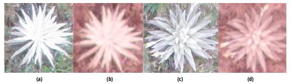
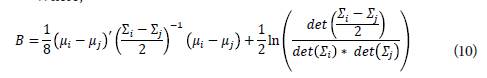
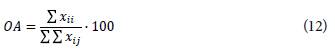
The study area lies in the moorlands of Chingaza [2], located in the eastern mountain range of Colombian Andes, from 3.100m to 4.700m a.s.l., towards the north-east of Bogotá D.C. Chingaza is considered as one of the most important moorlands because it provides about 80% of the municipal drinking water to the capital of Colombia, (Bogotá D.C.) [18]. The area of interest, which extends for half a hectare, was covered by capturing images using a UAV TAROT 680 PRO (with GPS and INS included). A total of 167 photos were acquired. Five ground control points were pre-signalized (4 located in the corners of the study area and the last at the Center) and positioned with a receiver GNSS Gr-5, in order to adjust the block of images. The UAV overflew the area 20 meters above ground level and was equipped with two Canon A2300 digital cameras. The first camera captured in the visible spectrum (400-700 nm) obtaining true color images (i.e. Red-Green-Blue - RGB combination), whereas the second camera was modified to capture in the infrared spectrum acquiring standard false color images (i.e. Near-Infrared-Red-Green - NIR combination). The data set was acquired in August 2016, with a Ground Sample Distance (GSD) of approximately 2 cm. The block adjustment of the images was processed with Pix4D * software. Figure 1 illustrates a sample of healthy and unhealthy Espeletia plants using both RGB and NIR. In 2017, Sastoque et al. [19] showed that differentiation of the biotic stress in Espeletia is evident in the spectral response captured in images acquired at different ranges of the electromagnetic spectrum, including the visible (true color images fig. 1a and 1c) and infrared (false color images fig. 1b and 1d).
Source: Author
Fig. 1 Healthy Espeletia plant vs. unhealthy plant. (a) Unhealthy plant in RGB. (b) Unhealthy plant in NIR. (c) Healthy plant in RGB. (d) Healthy plant in NIR.
On the other hand, texture analysis, specifically first order statistics and GLCM was performed in the ENVI* 5.3. software; while FT was done with PCI Geomatics* 2017 software. An Intel Core i7 processor with 6 GB RAM memory and operating system Windows 10 (64-bits) was used as computer system.
2.2 Proposed method
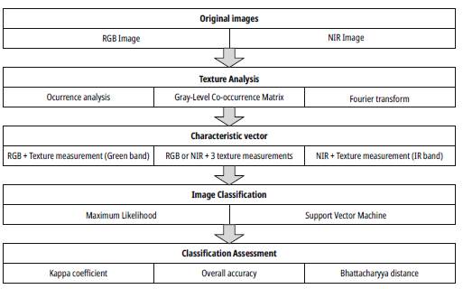
The complete process consists of four stages from the acquired images (RGB and NIR). Workflow is shown in figure 2. First stage is responsible for calculating the texture measures. In the second stage, characteristic vectors are generated from original images together with texture measurements. Third stage classifies the characteristic vectors to identify biotic stress of moorland Espeletia. Last stage assesses the classification of phytosanitary status of Espeletia plants.
2.2.1. Texture analysis
The literature review shows that the mean (MEA) and the variance (VAR) are the most appropriate first order statistics to describe the texture [12], [13], [16] and [32]. Likewise, in the Gray-Level Cooccurrence Matrix (GLCM), the contrast (CON), the entropy (ENT) and the correlation (COR) [9] - [11], [14], [16] and [32] are the measures that significantly improve the classification accuracy. Regarding the digital transformations, Fourier transform [24], [25] -including its special cases such as Gabor Transform [15], [24]- is one of the most commonly used methods for textural analysis. Therefore, based on the multispectral images, both RGB and NIR, texture measurements are applied, namely, MEA, VAR, ENT, CON, o, and FT. The window sizes selected here were 5x5, 11x11 and 15x15.
2.2.2. Characteristic vector
Once the textures features are created from the application of texture measurements, characteristic vectors are obtained for classification as follows: each original image (RGB and NIR) paired with each texture measurement (MEA, VAR, ENT, CON, COR, and FT), and evaluated for each of the window sizes (5x5, 11x11 and 15x15) [13], yields a total of 46 combinations. It is important to mention that, for the case of RGB original images, special attention is given to the Green band [9], [13]; and for the case of NIR original images, the emphasis was placed on the infrared band [9]. In case the three bands of the texture have been used, this is expressed in the vector of characteristics with the nomenclature RGB_3 or NIR_3.
2.2.3. Image Classification
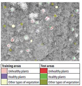
The choice of SVM as a classifier was due to the fact that it is considered a state-of-the-art automatic learning method and is increasingly used [5], [6], [12], [15]-[17]. Besides, SVM classification showed that it is possible to differentiate between biotic and abiotic drought stress in tomato plants [5]. Regarding ML classification is one of the most common methods [30]. Thus, the previous combinations are used to create the characteristic vectors that become the training set for both the ML and SVM classifiers. Thirty samples (fig. 3) were selected as part of the training set to create the characteristic vector that allows identification of the healthy/ unhealthy Espeletia plants as well as the areas with other types of vegetation [33]. The recognition of the phytosanitary status of Espeletia (both in the field and in the images) was identified in the guided tour carried out by the forest rangers of the moorlands of Chingaza at the time of the acquisition of images. The sample was composed of 911 pixels of healthy plants, 675 pixels of unhealthy plants, and 22208 pixels of other types of vegetation. Te samples were used in a systematic fashion in the forty-six classification rounds for each type of classification, namely ML and SVM.
2.2.4. Classification Assessment
In terms of assessment and validation of the classification results, nine samples were selected to validate the information (30% of the number of training samples). Visual interpretation was taken as the reference for validation. The same samples were used in all classification processes. Each of the 46 classified images is assessed using OA and K so as to determine their contribution, in termsof texture measurements, to the correct classification of the phytosanitary condition of Espeletia plants. On the other hand, the Bhattacharyya distance is calculated with the characteristic vector that offers the best results in the classification, that is, the classification that reaches one of the highest values of kappa.
2.3 Texture analysis
Two main categories of texture analysis are namely statistical and model-transform approaches.
2.3.1 Occurrence analysis
Occurrence analysis is done through the first-order statistics, calculated from the original values of the image, and do not consider the neighborhood relations of pixels. The most common statistics are the mean (Eq. 1), the variance (Eq. 2), the asymmetry coefficient, the kurtosis, among others [25-26].
Where, I is the random variable that represents the gray levels of a region of the image. This region of the image is a square matrix of size NxN.
2.3.2 Gray-Level Co-occurrence Matrix (GLCM)
GLCM belongs to the kind of statistical methods and consists in estimating image properties that arerelatedto therelative frequencies among gray levels (i.e. comparison of gray level frequencies) within the area of a predefined image window [10] [22].Haralick et al. [10] p ropose d 14 types of texture measu re ments th at can b0 extr acte d from GLCM. They include entropy (ENT - Eq. 3), contrast (CON - Eq. 4= and correlation (COR - Eq. 5).The expressions for texture measurements can be formally written as fo llows:
where P i,j is the normalized matrix of gray levels in celli, i, j,N is the number of rows or columns, σ t and σ i ; represent the standard deviation of row i and column j, respectively; µ t and µ j represent the mean of row i and column j, respectively. The entries of the normalized m atrix P i,j (E q. 6) a re g iven by th e following expression:
where Ci,j is the value of cell i,j in the matrix.
2.3.3.Fou rier transform
In the case of a discrete function (image) f (x, y) of two variables and NxN size, Fourier transform (Eq. 7) will be:
Fourier transform (FT) is a transformation tha tallows the calculation of the necessary coefficients so that the image can be represented in the frequency domain [20][27].Representations in this domaindetail how often certain patterns are repeatedin an image, managing torepresent the information of that image. This representation can be useful since having the frequency of repetition of such patterns can directly detect and alter elements present in the images, such as noise, contours or textures [27], [28].
2.4 Image classification
The information of multispectral images is gathered in the classification process, allowing the acquisition of cartographic information and the determination of the categories that will be studied [29]. In the present study, the categories correspond to healthy and unhealthy Espeletia plants. The remaining coverage areas will be classified as other vegetation. Within the classification process, three stages can be identified: i) category definition, ii) pixel distribution for the images in each category, iii) assessment and validation of results [29]. The categories can be defined, with or without the intervention of an operator, which corresponds to supervised and unsupervised classification processes, respectively. Pixel distribution is based on a simple assumption, namely, patterns are classified according to the degree of similarity to a specific prototype class or according to the nearest group center, using the concept of distance.
Maximum Likelihood classifier (ML) is one of the most popular methods of classification in remote sensing. It assumes that the data follows a normal distribution; thus a pixel is associated to the class that maximizes its probability function [29]. Support Vector Machine classification (SVM) is a supervised machine learning algorithm. It is a non-parametric method that uses the principle of structural risk minimization, aimed at minimizing the training error and does not assume a normal distribution of the data [29].
2.4.1 Bhattacharyya distance
The classes or categories considered to classify the images must be evaluated in order to establish the real separability of these categories. There are several numerical methods to estimate separability, such as normalized distance, statistical divergence, transformed divergence, Bhattacharyya distance , among others [30]. The distance of Bhattacharyya (BD - Eq. 9) is a very solid measure theoretically because it is directly related to the upper limit of the probabilities of classification errors [29]. Bhattacharyya distant between a pair of classes is defined as:
Where,
This measure of separability yields values between 0 and 2, where 0 indicates that the classes are superimposed, and 2 means that there is complete separability betwe n the classes. An empirical rule for interpreting the Bhattacharyya distance values is as follows: BD <1 indicates very poor separability, 1 <BD <1.9 indicates that the classes are separable to some extent and BD> 1.9 indicates high separability between classes [29], [31].
2.4.2 Confusion matrix
The confusion matrix is a square matrix of size n x n, where n indicates the number of categories considered in the classification. The rows of the matrix represent the reference categories (ground truth) and the columns, the categories classified. The diagonal of the matrix shows the number of verification points where the classified map and reality do not present discrepancies [30]. The residual values of the matrix represent the assignment errors committed in the classification: The residuals in the rows indicate the actual covers that were not included in the map (errors of omission), and the residual values of the columns indicate the covers of the map that do not conform to reality (commission errors).
From the confusion matrix, a series of statistical measures can be developed to evaluate the reliability of the map obtained. The simplest way is to calculate the overall accuracy (OA - Eq. 11), where the diagonal elements of the confusion matrix are related to the total number of sampled points x jj [30].
Kappa coefficient (K - Eq. 12) calculates the fit of the classified map and the reality observed in the terrain andeliminates the coincidences obtained in theclassification that could be caused by random effects [29].
Where, N: total number of reference pixels, xi+: marginal totals of row i, x+i: marginal totals of row j.
3. Results and discussion
Results are presented from three perspectives, namely: texture analysis, image classification and classification assessment.
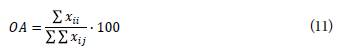
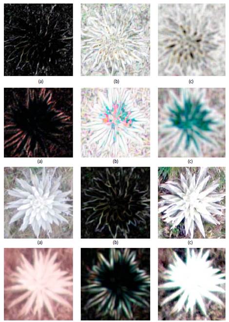
Regarding texture analysis, twenty-two characteristic vectors were generated (from both the original RGB and the original NIR image) according to their texture measurement and to their window size. Figure 4 is an example of the visual result obtained from applying different texture measurements to the images of healthy and unhealthy Espeletia plants.
Source: Author
Fig. 4 Texture measurements over images of healthy and unhealthy Espeletia plants. (a) Healthy Espeletia in RGB with CON and 5x5 window size. (b) Healthy Espeletia in RGB, with COR and 11x11. (c) Healthy Espeletia in RGB, with ENT and 15x15. (d) Unhealthy Espeletia in NIR, with CON and 5x5. (e) Unhealthy Espeletia in NIR, with COR and 11x11. (f) Unhealthy Espeletia in NIR, with ENT and 15x15. (g) Healthy Espeletia in RGB with MEA and 5x5 window size. (h) Healthy Espeletia in RGB, with VAR and 11x11. (i) Healthy Espeletia in RGB, with Fourier Transform. (j) Unhealthy Espeletia in NIR, with MEA and 5x5. (k) Unhealthy Espeletia in NIR, with VAR and 15x15. (l) Unhealthy Espeletia in NIR, with Fourier Transform.
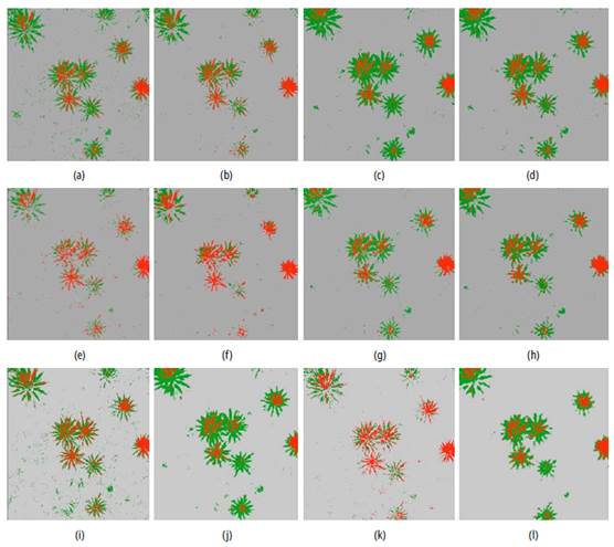
Concerning image classification, figure 5 shows a set of results obtained from the classification processes. In the figure, the red color indicates the presence of unhealthy plants, and the Green color is used for healthy plants; finally, the gray areas indicate the presence of other types of vegetation.
Source: Author
Fig. 5 ML vs SVM classification, unhealthy plants appear in red, healthy plants appear in green; gray areas represent other types of vegetation. (a) ML classification in RGB images. (b) ML classification in RGB images with ENT and 15x15. (c) ML classification in NIR images with ENT and 5x5. (d) ML classification in NIR images with ENT. (e) SVM classification in RGB images. (f) SVM classification in RGB images with ENT and 15x15. (g) SVM classification in NIR images with ENT and 5x5. (h) ML classification in NIR images with ENT and 15X15 (i) ML classification in RGB images with FT. (j) ML classification in NIR images with MEA and 5x5. (k). SVM classification in RGB images with 3VAR and 5x5. (l) SVM classification in NIR images with 3MEA and 15x15.
About classification assessment, tables 1 to 6 show the values of overall accuracy and Kappa coefficient obtained from the two classification processes (i.e. ML and SVM) for each of the forty-six images. Table 1 shows that the vector of NIR characteristics that includes the three bands of the mean in the 5x5 size yielded the best results with a Kappa coefficient of 0.9623 and an overall accuracy of 98.949%. Likewise, it is clear that the combination of the NIR image with the textural measurement of the mean in any size shows results better than those obtained with the variance. The behavior of the data is similar in the SVM classification (table 2).
Table 1 Accuracy assessment of occurrence analysis with ML classification in each image
| CHARACTERISTIC VECTOR | OA | Κ |
|---|---|---|
| RGB | 99.22% | 0.8673 |
| RGB_MEA 5 | 99.62% | 0.9305 |
| RGB_MEA 11 | 99.68% | 0.8437 |
| RGB_MEA 15 | 99.67% | 0.9387 |
| RGB_3 MEA 5 | 99.62% | 0.9307 |
| RGB_3 MEA 11 | 99.53% | 0.9142 |
| RGB_3 MEA 15 | 99.33% | 0.8816 |
| RGB_VAR 5 | 99.43% | 0.9000 |
| RGB_VAR 11 | 99.54% | 0.9156 |
| RGB_VAR 15 | 99.54% | 0.9157 |
| RGB_3 VAR 5 | 98.29% | 0.7464 |
| RGB_3 VAR 11 | 98.96% | 0.8224 |
| RGB_3 VAR 15 | 98.57% | 0.7688 |
| NIR | 98.68% | 0.8526 |
| NIR_MEA 5 | 98.82% | 0.9579 |
| NIR_MEA 11 | 98.85% | 0.9588 |
| NIR_MEA 15 | 98.79% | 0.9566 |
| NIR_3 MEA 5 | 98.95% | 0.9623 |
| NIR_3 MEA 11 | 98.66% | 0.9523 |
| NIR_3 MEA 15 | 98.48% | 0.9458 |
| NIR_VAR 5 | 97.49% | 0.9071 |
| NIR_VAR 11 | 97.03% | 0.8880 |
| NIR_VAR 15 | 97.15% | 0.8934 |
| NIR_3 VAR 5 | 97.33% | 0.9009 |
| NIR_3 VAR 11 | 97.14% | 0.8929 |
| NIR_3 VAR 15 | 97.45% | 0.9052 |
Source: Author
Table 2 Accuracy assessment of occurrence analysis with SVM classification in each image
| CHARACTERISTIC VECTOR | OA | Κ |
|---|---|---|
| RGB | 98.89% | 0.7595 |
| RGB_MEA 5 | 98.92% | 0.7774 |
| RGB_MEA 11 | 99.03% | 0.7904 |
| RGB_MEA 15 | 99.25% | 0.8437 |
| RGB_3 MEA 5 | 98.95% | 0.7820 |
| RGB_3 MEA 11 | 98.83% | 0.7556 |
| RGB_3 MEA 15 | 99.26% | 0.8457 |
| RGB_VAR 5 | 99.25% | 0.9193 |
| RGB_VAR 11 | 99.31% | 0.8748 |
| RGB_VAR 15 | 99.03% | 0.8210 |
| RGB_3 VAR 5 | 99.64% | 0.9305 |
| RGB_3 VAR 11 | 99.51% | 0.9056 |
| RGB_3 VAR 15 | 99.33% | 0.8666 |
| NIR | 97.76% | 0.8163 |
| NIR_MEA 5 | 98.04% | 0.9272 |
| NIR_MEA 11 | 98.74% | 0.9540 |
| NIR_MEA 15 | 99.07% | 0.9663 |
| NIR_3 MEA 5 | 98.88% | 0.9594 |
| NIR_3 MEA 11 | 99.47% | 0.9811 |
| NIR_3 MEA 15 | 99.51% | 0.9824 |
| NIR_VAR 5 | 96.81% | 0.8776 |
| NIR_VAR 11 | 96.61% | 0.8689 |
| NIR_VAR 15 | 97.09% | 0.8886 |
| NIR_3 VAR 5 | 96.95% | 0.8834 |
| NIR_3 VAR 11 | 96.93% | 0.8820 |
| NIR_3 VAR 15 | 96.97% | 0.8834 |
Source: Author
Regarding the results of GLCM (table 3 and 4), ENT offers the best results in both cases (SVM and ML classification). In the ML classification (table 3) the best results used all three texture bands, while in the SVM classification (table 4) the best results only used one texture band.
Table 3 Accuracy assessment of GLMC with ML classification in each image
| CHARACTERISTIC VECTOR | OA | Κ |
|---|---|---|
| RGB | 99.22% | 0,8673 |
| RGB CON 5x5 | 99.22% | 0,8712 |
| RGB CON 11x11 | 99.40% | 0,8871 |
| RGB CON 15x15 | 99.37% | 0,8782 |
| RGB ENT 5x5 | 99.70% | 0.9448 |
| RGB ENT 11x11 | 99.69% | 0.9440 |
| RGB ENT15x15 | 99.73% | 0.9495 |
| RGB COR 5x5 | 99.31% | 0,8807 |
| RGB COR 11x11 | 99.27% | 0,8748 |
| RGB COR 15x15 | 99.22% | 0,8669 |
| NIR | 98,68% | 0.9526 |
| NIR CON 5x5 | 98,81% | 0.9574 |
| NIR CON 11x11 | 98,37% | 0.9410 |
| NIR CON 15x15 | 97.70% | 0.9161 |
| NIR ENT 5x5 | 99.29% | 0.9745 |
| NIR ENT 11x11 | 99.14% | 0.9692 |
| NIR ENT 15x15 | 98,80% | 0.9570 |
| NIR COR 5x5 | 98.79% | 0.9566 |
| NIR COR 11x11 | 98,85% | 0.9587 |
| NIR COR 15x15 | 98,80% | 0.9570 |
Source: Author
Table 4 Accuracy assessment of GLMC with SVM classification in each image
| CHARACTERISTIC VECTOR | OA | Κ |
|---|---|---|
| RGB | 98,89% | 0.7595 |
| RGB CON 5x5 | 99.37% | 0,8836 |
| RGB CON 11x11 | 99.22% | 0,8567 |
| RGB CON 15x15 | 99.14% | 0,8435 |
| RGB ENT 5x5 | 99.43% | 0,8908 |
| RGB ENT 11x11 | 95,57% | 0.9113 |
| RGB ENT15x15 | 99.68% | 0.9393 |
| RGB COR 5x5 | 98,68% | 0.7027 |
| RGB COR 11x11 | 98,69% | 0.7055 |
| RGB COR 15x15 | 98,50% | 0,66 |
| NIR | 97.76% | 0.9163 |
| NIR CON 5x5 | 97,58% | 0.9089 |
| NIR CON 11x11 | 97.74% | 0.9152 |
| NIR CON 15x15 | 97,66% | 0.9131 |
| NIR ENT 5x5 | 96,66% | 0,8702 |
| NIR ENT 11x11 | 97,15% | 0,8911 |
| NIR ENT 15x15 | 98,41% | 0.9413 |
| NIR COR 5x5 | 96,83% | 0,8783 |
| NIR COR 11x11 | 96.94% | 0,8829 |
| NIR COR 15x15 | 97,08% | 0,8887 |
Source: Author
Accuracy assessment of Fourier transform (Table 6) shows that the NIR image yields a Kappa coefficient of 0.9722 and an overall accuracy of 99.230%, and in the case of the RGB image, a Kappa coefficient of 0.8788 and an overall accuracy definition of 99.298% is achieved. It is clear that the Fourier transformation improves the accuracy of the evaluation compared to the original data (RGB and NIR). In other words, the results are better for the SVM classification than ML classification (table 5).
Table 5 Accuracy assessment of Fourier transform with
| CHARACTERISTIC VECTOR | OA | K |
|---|---|---|
| RGB | 98.89% | 0.7595 |
| RGB_TF | 99.02% | 0.7985 |
| NIR | 97.76% | 0.8163 |
| NIR_TF | 97.31% | 0.8971 |
Source: Author
Table 6 Accuracy assessment of Fourier transform with SVM classification in each image
| CHARACTERISTIC VECTOR | OA | K |
|---|---|---|
| RGB | 99.22% | 0.8673 |
| RGB_TF | 99.29% | 0.8788 |
| NIR | 98.68% | 0.8526 |
| NIR_TF | 99.23% | 0.9722 |
Source: Author
By analyzing together figure 5 and tables 1 to 6, it is evident that OA is similar in all classifications, and an improvement in the classification is reflected in a better K.
Tables 7 and 8 show the distance of Bhattacharyya to evaluate the separability of classes in the characteristic vectors, namely NIR_3 ENT 5x5 (best classification in GLMC with ML) and RGB_3 ENT 5x5 respectively. Results show that only classes that will have a probability of being confused in the classification are the healthy Espeletia with the other kind of vegetation, because its values are lower than 1.9. With regard to unhealthy plants, theses cannot be confused with healthy plants, because distance of Bhattacharyya is higher than 1.9, so this means that they are separable. Thus, upon comparing results, Sastoque et al. [19] reaffirm spectral separability of healthy Espeletia versus unhealthy Espeletia.
On the other hand, by observing table 1 to 6, it is clear that the values of both OA and K, for the case of RGB images, improve when including texture measurements. A similar behavior can be observed for the case of NIR images. As to occurrence analysis, the best result was obtained in NIR_3 MEA 15, with OA = 99.51% and K = 0.9824. In regard to GLMC, the best result was achieved with NIR ENT 5x5, with OA = 99.29% and K = 0.9745. Finally, Fourier transform reached with NIR_TF an OA = 99.23% and K = 0.9722.
As regard GLMC, the highest values of OA and K were obtained from the ML classifier with ENT as the texture measurement. In the case of true color images, with parameters RGB, ENT, and 15x15, the OA value was 99.73%, while the value of K was 0.9495. Meanwhile, for the case of false color, with the NIR, ENT, 5x5 image, the OA value was 99.29% with a K value of 0.9745. Regarding the results obtained when including texture measurements COR and CON, for the case of RGB images, no window size yielded a value of K above 0.9. However, for the case of NIR images, K values were very similar to those obtained when no texture measurement was applied.
The results presented herein compare to those obtained in other studies in several ways. Regarding the texture window size, Feng et al. [13] indicated that the enlargement of the window size increases the accuracy until reaching an optimal texture scale; however, finding a formula to determine the optimal scale is cumbersome. In our case, most of the best results were obtained with a window size of 15x15; however, it was necessary to conduct different experiments with different window sizes to find the optimal scale that allowed identification of Espeletia. Despite this limitation, the inclusion of the texture in the characteristic vector led to an increase in the value of K in all cases (e.g. the case of occurrence analysis in the RGB images going from K = 0.7595 to K = 0.9303). Thus, in a similar way to the works of David and Ballado [9], Laliberte and Rango [11], Yue et al. [12], Feng et al. [13], Hashim et al. [15], Ferreira et al. [16] and Mishra [17], the incorporation of textural measures increases the classification accuracy remarkably.
Table 7 Bhattacharyya distance in the characteristic vectors NIR_3 ENT 5x5
| Healthy Espeletia plants | Unhealthy Espeletia plants | Other kind of vegetation | |
|---|---|---|---|
| Healthy Espeletia plants | - | ||
| Unhealthy Espeletia plants | 196.687.835 | - | |
| Other kind of vegetation | 184.510.403 | 199.969.828 | - |
Source: Author
Table 8 Bhattacharyya distance in the characteristic vectors RGB_3 ENT 5x5
| Healthy Espeletia plants | Unhealthy Espeletia plants | Other kind of vegetation | |
|---|---|---|---|
| Healthy Espeletia plants | - | ||
| Unhealthy Espeletia plants | 192.680.578 | - | |
| Other kind of vegetation | 183.021.412 | 199.969.828 | - |
Source: Author
Concerning the spectral separability of classes in the characteristic vectors, the results show that unhealthy Espeletia will not be mistaken by healthy Espeletia since the Bhattacharyya distance is larger than 1.9. These results compare to the study by Ferreira et al. [16], in which Bhattacharyya distance was used to verify whether the GLCM texture features influence the interspecific spectral separability of the species. Moreover, when including texture measurements in the classification process, the values of K and OA are similar (even better) to the values obtained with the SAM method (Spectral Angler Mapper), which makes use of field spectral radiometry [19]; this method yielded a K value of 0.772 and an OA value of 95.96% while our best result (NIR_3 MEA15) reaches a K value of 0.9824 and an OA value of 99.51%. These results allow proper identification unhealthy Espeletia.
In terms of biotic stress, similar to the works in Ondimu and Murase [14], Susi'c et al. [5] and Zibrat et al. [6], the use of remote sensing imagery techniques allows the identification and spatial location of the stress areas, namely biotic stress in Espeletia plants, as in the present study.
These results show that the use of textural measures on images acquired with UAV allows an improvement in the classification of the images [9], [12], [13] for the purpose of identifying biotic stress. The extent of the improvement permits a comparison with the results obtained by spectroradiometry in the field, which opens the possibility of reducing costs in field studies and allows the exploration of larger areas with shorter processes demanding less time. Additionally, the presented approach enables frequent monitoring of the area of interest given the possibility of revisit offered by UAV flights [12]. This type of analysis offers a preliminary approximation of the affected areas leading to timely decision-making for the improvement actions taken by thematic experts.
4. Conclusion
UAV-imagery (RGB and NIR images) were taken in an area of interest in the moorlands of Chingaza (Colombia). As a result of digital processing of UAV-imagery and their subsequent analysis, it was concluded that the inclusion of GLCM texture measurements into the spectral information of images significantly improved classification accuracy when identifying the presence of biotic stress in Espeletia plants. Texture measurement MEA yielded the best results for all classification processes, attaining an almost ideal matching, namely a K value of0.9824 and an OA value of 99.51°%. Likewise, the window size leading to the best results, when using the RGB and NIR spectral information, was 15x15. In terms of classification accuracy, the results were slightly better when using the SVM classifier, compared to the results obtained with the ML classifier. Likewise, better classification results were obtained from NIR images when compared to those from RGB images.
The use of textural measures for the identification of phytosanitary status of Espeletia, is presented as an alternative for monitoring the biotic stress that this kind of vegetation has been presenting in recent times, because it allows identifying potentially affected areas so that specialists of the subject can take (preventive or corrective) actions in order to preserve the species Moreover, images can be taken with the desired frequency, thus monitoring can be carried out as regularly as the specialists may require.

