


 English (pdf)
 Article in xml format
 Article references
 Send this article by e-mail
 Cited by SciELO
  Cited by Google
  Similars in
SciELO
Similars in
SciELO  Similars in Google
 Permalink
Introduction
Representing chemical processes, commonly called modeling, has been done since the very beginning of process engineering based on three kinds of models: verbal, graphical, and mathematical, and their various combinations. However, mathematical models are mostly used due to the accuracy needed in the engineering processes and the wide availability of analysis tools.
There are three families of mathematical models: i) phenomenological/white box or mechanistic models; ii) empirical or black-box models, and iii) semi-physical or gray-box models. This last family includes two sub-families, the phenomenon-based semi-physical models (PBSM) and the empirical semi-physical models. PBSMs are the most commonly used in process engineering (Aris, 1994; Hangos & Cameron, 2001).
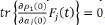
This type of mathematical model is used in systems conceived as a part or abstraction of the real process. To understand the dynamics of a system with a large number of particles and be able to predict new events in the future, attention should be focused on the scale chosen to develop the mathematical model. At this point, it is possible to refer to microscopic scales where the dynamics are governed by a mathematical model based on Newton's classical dynamics equations or on the Hamiltonian scheme, which would allow finding the position and the speed of the N particles of the system and then measurable magnitudes such as temperature, pressure, density, energy, etc. by taking the average based on the distribution function of macrostates. Sometimes, this last operation is very difficult given the huge number of initial conditions and equations to solve.
On the macroscopic scale, the model represents the process as a lumped parameter with the option of considering the local effects and time variation (possible spatial macroscopic partitions). The system is modeled considering that each macroscopic part of the system evolves at the same time, i.e., each variable featured by density varies uniformly in time and into a given partition in space. These partitions, commonly of macroscopic size, are arbitrarily taken by the modeler with the option of taking cellular sizes too. The macroscopic scale for these kinds of models is also called the thermodynamic scale.
Both the microscopic and macroscopic approaches have limitations when used indi vidually to construct a process model. There is a big gap between their time and length scales, which leads to a fragmentary representation of some chemical processes when the system has high anisotropy, reflects complex phenomena, or includes new physical phenomena poorly known as functions of the ensemble. Such ignorance is explained by the fact that some phenomena are only visible in the partition size. These limitations are associated with the impossibility of explaining certain measurements of the process at the microscopic scale or the lack of knowledge regarding transport coefficients at the macroscopic scale, which demands a larger spatial and temporal scale known as the mesoscopic scale (Figure 1) where clusters or sets of particles are taken as if they were individual points or macroparticles associated with a motion equation that should be developed to describe the system dynamics from new variables as the mass, the momentum, and the energy density.
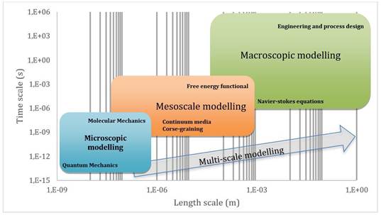
Here we explore the mesoscopic scale models as a link between the micro and macro worlds and the way dynamic equations have evolved as a function of relevant information in modeled processes to close the gap and open the way to the construction of a multi-scale model. This proposal is supported by the basic concepts of the mathematical process model for each scale level. The main novelty of our work, therefore, is that, for the first time, the general procedure to propose mathematical models at different scales considering the connection between them is developed in a systemic and orderly manner, which usually is not explicitly presented in scientific literature.
Suggested modeling procedure for macroscopic scale
To obtain a phenomenon-based macroscopic model, we propose the following methodology (Álvarez et al., 2009; Lema-Pérez et al., 2019), which has been used for the design of several phenomenon-based semi-physical models (PBSM) (David et al., 2020; Zuluaga-Bedoya et al., 2018). It consists of 10 steps divided into three stages: model pre-construction (steps 1 to 3); model construction (steps 4 to 7), and model simulation and validation (steps 8 to 10). The procedure was developed by interacting with model users and reviewing published procedures such as those of Basmadjian et al. (2007) and Hangos & Cameron (2001). We reviewed 21 procedures in total (Ortega-Quintana et al, 2017) with the aim of simplifying some steps and looking for a direct sequence easily applicable by junior researchers.
The steps are the following:
Describe the process and state the model objective. Formulate verbally the question to be answered by the model and sketch a complementary process flow diagram (PFD). A poorly understood process conducts to an erroneous model. The description should be detailed enough but avoid irrelevant aspects of the real process. The verbal description and the PFD are refined during the construction of the model.
Formulate the modeling hypothesis and the level of detail. Define the operation and the phenomena taking place in the actual process, or an analogy for it. An analogy is knowledge-based guesswork where imagination should be used to describe what is unknown, obviously resorting to what is known, which means it does not run free. Thus, the description of the unknown aspects gains similarity from a known object and the behavior of the unknown portion that is measured can be predicted based on what the imagination builds as the phenomena take place. Following this line, the modeling hypothesis is a brief description of the real or supposed way in which a number of known phenomena interact to make the real process come true.
When formulating the modeling hypothesis, it is possible to ease one or more known phenomena conditions and adapt them to describe the aspect of interest of the real process. To this aim, a set of assumptions justifies the assembly of known phenomena in the real process or the analogous one. Given the permanent review of the modelling hypothesis during the development of the model, some assumptions may change.
Moreover, to construct a model, the real process should be partitioned to observe process parts and their interactions. In the case of PBSM, these parts are called process systems (see next step). According to the model objective or purpose, a certain level of detail should be stated as well to define the position of the relevant part in a useful real engineering size scale. Such a scale begins with gross details indicating the real object and ends at the minimum physical size to be used in the modelling process. Clearly, steps 1 and 2 are a loop susceptible to permanent improvement during model development.
Define process systems (PS). The partition of the process consists of defining as many process systems (PS) as required by the level of detail. A PS is the abstraction of a part of the process as a system, i.e., all the available tools of systems theory and system engineering can be applied to that part (Hangos & Cameron, 2001). To determine a PS: a) Look for physical walls in the process. The two volumes separated by a wall could be considered two PSs; b) detect distinguishable phases of substance within the same volume and assign a PS to each phase regardless of one being dispersed and the other the continuous phase (Zuluaga-Bedoya et al., 2018); c) detect any mass characteristic marking spatial differences and separate each portion of the mass with similar characteristics as a PS (Atehortúa et al., 2007), and d) use arbitrary limits when the PSs obtained are useful for model development (Hoyos et al., 2016). Finally, a block diagram relating all PSs should be plotted.
Apply the conservation principle to all declared PSs. Apply the conservation principle to each PS defined to obtain the equations from which the model's basic structure will be extracted. It is recommended to take at least these balances for each PS: a) total mass, b) n-components mass, c) thermal energy, and d) mechanical energy or momentum. These equations form the balancing equations (BE) set, which is a non-minimal set as some of these equations give the same information, and, therefore, some of them can be discarded from the model's basic structure.
Determine the model's basic structure (MBS). Select the set of equations rendering information that will fulfill the model's objective (Step ii.) from previously found balancing equations (BE) and constitute the model's basic structure. All redundant equations are then excluded from the model's basic structure.
List MBS variables, parameters, and constants. Establish the variables, parameters, and constants of the model. There are several alternative interpretations in published works of the term "variable", which, to avoid confusion, should be differentiated from the term "unknown parameter", commonly used to evaluate the degrees of freedom of a set of equations (see Step viii). Model variables are a part of mathematical model unknown parameters but not all of these are variables. All parameters are unknown for the mathematical set of equations forming the model. Steps vi, vii, and viii form a loop but they appear as a sequence in the final procedure.
Propose constitutive and assessment equations for model parameters. Propose or find constitutive and assessment equations in the literature to calculate the largest number of parameters in each PS. This is the most critical step because the modeler must arbitrarily choose equations to represent the model parameters. For those with no constitutive or assessment equations, the modeler should identify a value from experimental data (Ljung, 1999). At least one of the parameters identified can act as a fine tuner of model response (Lopez-Restrepo et al., 2020). A constitutive equation approximates the response of a physical quantity to external stimuli using a law or principle, for example, the Arrhenius law. In turn, an assessment equation is a mathematical relation to assess a parameter value with no intention of linking the calculated value to the phenomena in a descriptive way. A constitutive or assessment equation for a given parameter can produce new ones, which must be determined too. These are located deeper in parameter structure layers, i.e., they are lower in the level of specification of the model. It should be considered that the specification (evaluation) level is different from the detail (size) level.
Determine the degrees of freedom. Verify the degrees of freedom (DF) of the model's structure: mathematical systems formed by all model equations (basic and extended structures). The DFs are the difference between the number of unknown parameters and equations and it must be zero for a solvable model.
Build a computational model. Build a computational model or computer program capable of solving the model equations without altering the true mathematical model response. The required computational model translates the model extended structure to a computational code capable of solving the PBSM. Again, the lumped or distributed parameters characteristic of the model must be considered during computational model construction (Wendt et al., 2009), as well as an appropriate discretization methodology to represent continuum fields as a system of algebraic equations. Discretization strategies based on Eulerian and Lagrangian schemes can be found for this purpose.
Validate the model. Validating the model response is the last step of the procedure. The idea is to contrast the model-predicted values with real data taken from the process under the operating conditions established in Step ii for the model objective. If real process data is not available, it is possible to validate the model response against the expected behaviour of the process in accordance with available knowledge regarding similar processes. In this sense, the main behaviour of the process should be reflected in the model responses.
Suggested modeling procedure for the mesoscopic scale: Closing the gap
In nature, physical systems are composed of many identical constituents at the microscopic level that impact the dynamics of the variables at the macroscopic level. However, macroscopic systems exhibit a relatively simple behavior described by motion equations for a few reduced variables: commonly, a state function in the phase space is established through the sum of individual state effects to get an average. These averages change slowly over time and can be measured at the macroscale. Regarding the two basic scales, the connection between the microscopic scale and an intermediate one -called mesoscopic- is of interest to several scientific and academic disciplines. The statistical mechanical theory has tried to find a suitable link between both worlds to relate this mesoscopic dynamic with the underlying microscopic process. One of the advantages of working at the microscopic level is that the process has reversible dynamics entirely determined by the Hamiltonian H and the initial probability density p(t o ), from which all properties of the system can be calculated, at least in principle.
On the other hand, at the macroscopic scale, the transport equations describe the evolution of a non-equilibrium system (e.g., the Navier-Stokes equations for fluids, the Bloch equations for magnetic relaxation, the Fokker-Planck equation for Brownian particles, and the master equation for atoms interacting with a radiation field), and the fundamental transport equation (e.g., Fick, Fourier, Newton) representing the thermodynamic potential. Two parts conform to these dynamics equations: one relates to reversible processes and the other is the irreversibility generated by the underlying molecular nature. The first one has a Poisson bracket structure whereas the second is related to correlations of instantaneous microscopic fluxes (Camargo et al., 2018; Español, 1993; Español et al., 1999). Several authors, from Einstein (1905) to Kirkwood (1947), Kirkwood et al. (1949), and Onsager (1931), noticed the intimate connection between fluctuations and irreversible behavior in non-equilibrium systems, which open the way to the design of irreversible processes thermodynamics (Groot & Mazur, 1984). The Gauss-Markov processes crystallizing in Onsager's reciprocal relations (Onsager, 1931) and the fluctuation-dissipation theorem (Green, 1954; Kubo, 1957) are examples of this connection.
The uncertainties resulting from the elimination of degrees of freedom when changing from the microscale to the macroscale generates fluctuations and dissipation, which can be related to the fluctuation-dissipation theorem or correlations of microscopic fluxes using the Green-Kubo-type formulae under the Markovian assumption (Español, 1993; Torre et al., 2019). The latter is essential for defining transport coefficients to close the motion equation and connect the scales. The transition from a microscopic scale to a macroscopic one has been achieved by projecting the dynamics in slow states and their fluctuations. This is a stepwise process in which the hierarchical path from the world to the micro-world, as fully identified by the Liouville equation, and then to the macro world fully identified by the Navier-Stokes hydrodynamic equation. Thus, it is a compelling way of linking both worlds. However, everything occurring at the microscale depends on the system's external perturbation.
Using the Liouville equation at the microscale and the Navier-Stokes equations at the macroscale apparently enables a quick jump from microscopic dynamics to the macro-scale. However, this is accurate only for physical systems known as "ideal fluid" or "simple fluid", i.e., systems with full isotropic transport kernel conditions and homogenous chemi cal composition. Additionally, the poor physical and mathematical connection between these two models makes it difficult to develop a discretization scheme for hybrid models (Donev et al., 2010a; Donev et al., 2010b). Therefore, this approach is difficult to fulfill in chemical processes (multi-compound processes) or complex fluids, which despite their continuum appearance at macroscopic scale present a non-equilibrium structure, nanoscale anisotropy, or coupling between the fluid structure and the flowing properties. Therefore, a new multi-scale strategy to model chemical processes should be evaluated to translate flawlessly the information between the different scales and allow a stable mathematical connection between dynamic equations at different scales (Figure 1).
An intermediate scale called mesoscale has arisen to achieve the multi-scale modeling and overcome the above-mentioned problems as its temporal and length scales are higher than the microscale but lower than the macroscale. However, as time and length increase, the collective motion will hide the erratic movements and particle collisions predicted by microscopic models. Besides, the local equilibrium, isotropic fluid, and smooth density gradient, among other assumptions in the continuum media, are not guaranteed, and the time scale dynamics are faster than in the macroscale. Although each phenomenon may have times and scales, the state-of-the-art can help define an expected range in the mesoscale from 1 ns to 106 ns for time and from 5 nm to 105 nm for length (Ellero & Español, 2018).
The applied mesoscale models started with two popular techniques. The first one is the top-down technique, which aims at addressing the non-equilibrium, non-locality, and hydrodynamics anisotropy, among other complex behaviors on the dynamic equation, by including thermal fluctuation in Navier-Stokes equations (Bell et al., 2007; Landau & Lifshitz, 1959, 1987; Mansour et al., 1987; Mashiyama & Mori, 1978; Voulgarakis et al., 2010)(de Zárate & Sengers, 2006). As a result, the mesoscopic hydrodynamics are represented by stochastic differential equations (SDE) with a stochastic flux for the stress tensor, the heat flux, and the diffusion flux while relevant variables are preserved through fluxes divergence.
The second technique, the bottom-up technique, represents the dynamics of a set of big clusters or fluid regions moving in continuous space and discrete time. Therefore, a new set known as "the relevant variables" appears to act as a set of microscopic particle aggregation in a new subsystem called a cluster, micro-continuum cell, or coarse-grained dynamics that need specific dynamic equations. The "coarse-graining" methodology is used to reduce a set of individual small particles (atoms or molecules) to one particle with the mean feature and a reduced force interaction representing the set interaction (Avalos & Mackie, 1999; Español, 1995; Español et al., 1997, 1999; Español & Warren, 1995; Hoogerbrugge & Koelman, 1992). One of the main advantages of this procedure is that relevant variables in the mesoscale move slowly over time and cover larger sizes, so it is possible to measure them with modern techniques and low processing information cost (time and resources).
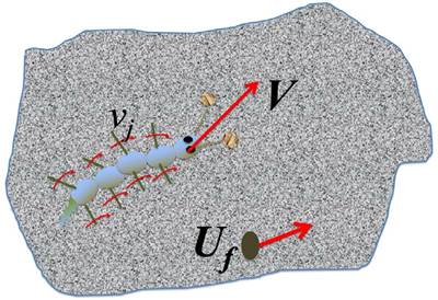
A metaphoric example of the validity of macroscopic systems analyzed with slow and observable variables is a worm with many legs moving ( ). The worm dynamics can be analyzed based on the observation and monitoring of the position based on the v-velocity regardless of the movement of its multiple legs. However, the information on the dynamics of the legs can slightly alter the physical trajectory of the worm, thus generating oscillations or fluctuations.
One of the most popular tools applied to the coarse-graining concept is the dissipative particle dynamic (DPD) (Vishnyakov et al., 2012; Du et al., 2015; Cao et al., 2005) because it allows the representation of the larger-scale dynamics of a stochastic particle having soft conservative, dissipative, and random contributions. However, this tool doesn't count with dynamic energy or entropy equations, or physical size relation (Ellero & Español, 2018). Such SDE models can be framed, then, with a coarse-graining technique based on the Fokker-Plank equation representing the dynamics of a probability distribution of mesoscale variables. Under this precept, Lagrangian models have been developed with smoothed dissipative particle dynamics (SDPD) and smoothed particle hydrodynamics (SPH), for example (Ellero et al., 2007; Español et al., 1997; Español & Revenga, 2003; Monaghan, 2005; Vázquez-Quesada et al., 2009). However, in the last decade, a significant evolution of the mesoscopic model strategy has been developed to find a well-defined physical and mathematical support for the coarse-graining techniques and reduce the possibility of models based mainly on the builder's expertise. This approach is used to close the gap between microscopic and macroscopic modeling.
Relevant variables and their general motion equations at the mesoscopic scale
The reduction of microscopic variables
 to collective-field variables is the first step in the transformation of microscale into meso- and macroscales (bottom-up approach). These new relevant variables capture the joint motions of atoms or molecules. Today, this step has become routine thanks to the relevant works of Einstein (1905) and Onsager (1931), the extensive work of Kirkwood (Irving & Kirkwood, 1950) in Markoff random processes, and the statistical mechanics of time-dependent phenomena of MelvilleGreen (1954) and RyogoKubo (1957), among others.
The transport equation on the mesoscopic scale governs the dynamics and accounts for the evolution in time of the behavior of nature. The equation results from knowing the information at the lower scale, which is challenging because the system contains many particles or degrees of freedom. Therefore, the concept of thermodynamic assembly is used coupled with the separation of slow dynamics of high relevance (relevant variables: numerical value {a. (t)} of an invariant function
 ) and fast dynamics of little significance. Here,
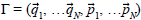
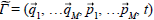 is the reduced phase space of
 ) where M << N.
It would not be possible to define or build the distribution function (classic) or density matrix (quantic) p(r, t) in detail. Therefore, the value of a set of relevant variables {a
j
(t)} can not be determined entirely in a non-equilibrium state at time t. To predict the evolution of the system, it is necessary to capture the value of a property ({a
j
(t)}) by performing many tests or attempts, which would require the mean values of a complete set of variables; hence, it is essential to introduce a probability distribution
 in the subspace of the numerical value {a
j
(t)} of an invariant function
in the subspace of the numerical value {a
j
(t)} of an invariant function
 , which is only a function of these values {a
j
(t)}. The probability at the time t of this event is:
, which is only a function of these values {a
j
(t)}. The probability at the time t of this event is:

There is a distribution probability g(a j (t)) of having the specific value of {a j (t)}. First, we have the microscale with the possibility of the state (ensemble) to translate the world seen as a set of states in the microscale to another one seen as a set of mean values of the phase function characterized by a probability function. In the end, it is easy to translate it into another world identified by the average {a j (t)} of the mean values of the phase functions.
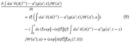
At this point, it is necessary to find the dynamic equations to compute the new variables a j (t) or g(a j (t)), which we will call the motion equation or transport equation. To do so, the projection operator (P) method is used to divide an ensemble density or distribution function (p(t)) into "the relevant" part (p 1(t)) and "the irrelevant" part (p 2 (t)) (Zwanzig, 1960, 1961):

where

and

The relevant probability density p 1(t) defines the microscopic system clearly and exactly by taking a few relevant variables as in the mesoscopic world. The idea of the projection operator approach is to express the relevant ensemble as a result of a projection P acting on the real ensemble Pp(t), and the irrelevant ensemble as a function of the relevant one presented in Eq. (3), which simplifies the understanding of the dynamic of nature without losing the information. Moreover, it is an approach that reduces a world with many variables to one with fewer relevant variables.
The microscopic time evolution operator is decomposed with the help of the projection operator into a sum of three terms: the first one is wholly determined by the instantaneous values of the macroscopic variables; the second one by their history and the third term is of microscopic origin and leads to the irregular motion of macroscopic quantities. Therefore, the operator projection can be defined also as proposed by Zwanzig:
where p
1(Γ, t; a) is the projected functional part on a specific area of the phase space that takes the value of a, while
 is the structural function of subspace or when
 = a.
= a.
The projection operator takes advantage of the interesting value of the states that are enough to explain the behavior of nature and leaves out the variables that are not impacted at the same time scale. By applying the operator projection to Liouville's equation, we can write a pair of equations:
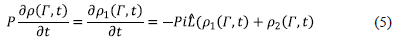

These equations can be solved formally by p 2(Γ, t) in terms of p 2(Γ, 0) and p 1(Γ, t):

Then we can replace (7) with (5):

and take the definition of p 1(Γ, t) as indicated in (4) to obtain:
solving the first integral on ∫ da':
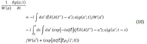
The fluctuation term
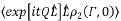 is neglected because on average fluctuations it is neglected at equilibrium and is the same as Pp(Γ, 0) = p(Γ, 0). The projection operator specifies an initial ensemble density to guarantee the validity of this assumption. In this way, these terms are not considered. Now, taking the definition of p
1
(Γ, t) or (4) in the subspace of value a and putting it into (10):
is neglected because on average fluctuations it is neglected at equilibrium and is the same as Pp(Γ, 0) = p(Γ, 0). The projection operator specifies an initial ensemble density to guarantee the validity of this assumption. In this way, these terms are not considered. Now, taking the definition of p
1
(Γ, t) or (4) in the subspace of value a and putting it into (10):
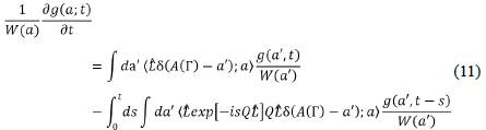
we can derive the transport equation for the mesoscopic variable (α
j
(t)) in the physical space by doing the average a, (t). We reduced the problem to the physical world

 because we took the integral on all the moments of the variables. For doing so, (11) is multiplied by α
j
and then it is integrated using
because we took the integral on all the moments of the variables. For doing so, (11) is multiplied by α
j
and then it is integrated using
 and taking into account the definition for thermodynamic force as
  the transport equation becomes
The change of a mean value over time consists of two terms:
The first term describes organized mesoscopic motion. The expression for this term could be the classical hydrodynamic or Navier-Stokes equation without the irreversible or dissipative terms of the mesoscopic scale evaluated at the present time t. With this term, the future dynamics are determined by the current value of the variables.
The second term corresponds to the irreversible or dissipative terms due to the microscopic dynamic revealed in the mesoscopic equation of motion as a flux term,
 . Its future dynamics include the past or memory term if we do not consider the Markovian process:
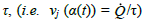
As shown in (4), transport coefficients (K jk (α (t - s); s)) and forces ((α (t - s))) depend on what happened in the past (0 « s « t). Likewise, the generalized Langevin equation can be derived from (12) by assuming the second term in the integral as a stochastic force:
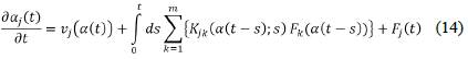
Equation (14) can be written in a compact form as:
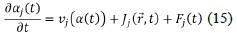
where F
j
(t) = δF
j
(0, t) = F
j
(0, t) = Q(0) G
0,t
ȧ
j
with the following property 〈F
¡
(t)〉 = 0 and
 . The generalized Langevin equation determines the stochastic process of the macroscopic variables in terms of another process, the stochastic process of the random forces F(t), which means we must know them to determine the stochastic process of the fluctuations. However, their evaluation is very complicated since the parts of the transport coefficients with a delay K
mk
(t, u) and the correlations of the random forces <F
i
(t)F
j
(s)> are given in terms of involved molecular expressions.
. The generalized Langevin equation determines the stochastic process of the macroscopic variables in terms of another process, the stochastic process of the random forces F(t), which means we must know them to determine the stochastic process of the fluctuations. However, their evaluation is very complicated since the parts of the transport coefficients with a delay K
mk
(t, u) and the correlations of the random forces <F
i
(t)F
j
(s)> are given in terms of involved molecular expressions.
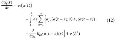
Equations (12) and (14) reveal the main phenomena visible at mesoscopic scales due to the collective effects of the interactions between particles, which can generate a memory effect depending on how fast the phenomenon occurs. Therefore, the time change of any relevant variable depends on its mean values and the correlations between its fluctuations, i.e., the variation on time of any relevant variable a m (t) depends on the mean value at the present time, the correlation of the fluctuation that happened in the past, and the stochastic information due to unknown events as from the initial time. These closed equations of motion display the universal structure of exact equations in non-equilibrium statistical mechanics. However, their solution is possible only in an approximate way.
These expressions are relevant given the connection between the different scales both in time and space. The connection between the microscopic and mesoscopic worlds can be appreciated through the memory effect term K mk (t, s) and the random force term F m (t) perceivable when there is an increase in both the length and time scales of the system.
The reversible part (first term of Eq. 12)
Extensive elements such as nanoparticles, nanopores, or complex reactions can affect the fluid isotropy to generate a complex system that must have a dynamic equation. But then, what happens to anisotropic systems? How to change the dynamic equations? These are questions that should be answered. In contrast with the micro- and macroscale models, at the mesoscale, the system may be described at different levels as a function of the set of relevant variables defining its state, the reduced information (or captured information), and a temporal characteristic scale of the dynamics. The degrees of freedom eliminated or uncertainties are considered a systematic dissipative effect of the relevant variables, i.e., the transport coefficient.
Therefore, the mesoscale has various levels of description with a specific dynamic equation as a function of the physical system and the time-space scale to be modeled. Figure 3 summarizes the description routes and levels required to model the mesoscale in the most common physical systems: the colloid suspension and the single fluid. The common starting point in both cases is the hydrodynamic or average level, which shares the statistical-mechanical collective field variables described as mass density, momentum density, and energy density. Its main aim is to change the discrete world of individual particles into continuum variables to establish their dynamic equation and transport coefficient. Here we hope to define the non-local transport coefficient reducing the fluid anisotropy by interacting with the macromolecules, walls, and other elements in the boundary condition of fluids or macromolecules dynamic equations.
A second level of description in mesoscales is the Fokker-Planck level (Eq. (10)). Using the stochastic dynamics of the system the thermal fluctuation, drag, and random forces are considered a result of eliminating fluid or macromolecules degrees of freedom. Additionally, the fluctuation and dissipation theorem constitutes a frame of stochastic sources for the dynamics of the relevant variables.
Finally, we can consider an additional description level of macromolecules immersed in the fluid before reaching the macroscale, which is known as the Smoluchowski level, and is a particular case of the previous level; the change of position of the macromolecule is lower than that of other variables as a momentum of both fluid and macromolecule. Therefore, the probability distribution function of the macromolecule position can be reduced to a simpler stochastic dynamic such as that of the Langevin equation (Eq. (12)). The Brownian motion assumption is a precise application of this mesoscopic level of description.
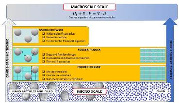
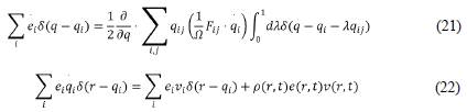
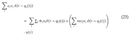
Let us consider the transport equation for the mesoscale scale as a hydrodynamic equation using the coarse-grain concept where the relevant variables are mass density field p(r, t), momentum density fields p(r, t) u(r, t), and energy density fields p(r, t) e(r, t) defined as an Eulerian picture in that position r; therefore, the relevant variables A j are:
where p(r, t) = 1/Ω Σ
i
m
i
δ(r - q
i
(t)) is the matter per volume unit or density, p(r, t) u(r, t) = 1/Ω Σ
i
P
i
δ(r - q
i
(t)) is the momentum per volume unity, p(r, t) e(r, t) = 1/Ω Σ
i
e
i
- δ(r - q
i
(t)) and e
i
= 1/2 m
i
v
i
2
+ 1/2 Σ
j
ϕ(q
ij
) are the energy per volume unity in phase space with reduced state variables, m
i
represents the atomic or molecular mass, and u(r, t) is the stream velocity of the system. This coarse-grain variable is closely related to the microscopic velocity of a particle i
th
v
i
and the global velocity
 while δ is the Dirac's δ-function; the probability by unit of volume that the i
th
molecule is at r and time t, also known as the coarse-grain delta function, supports the finite small region and is normalized to unity (Español et al,
1999). Therefore, it is possible to obtain the microdynamic equations from density fields in the reference system position r by:
while δ is the Dirac's δ-function; the probability by unit of volume that the i
th
molecule is at r and time t, also known as the coarse-grain delta function, supports the finite small region and is normalized to unity (Español et al,
1999). Therefore, it is possible to obtain the microdynamic equations from density fields in the reference system position r by:
Mass density field
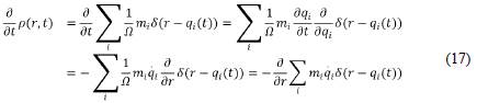
Momentum density fields
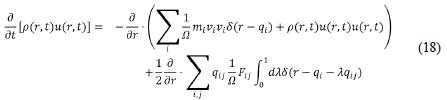
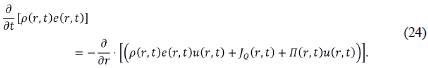
where the pressure tensor Π (r, t) is represented by
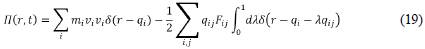
and the energy density fields by
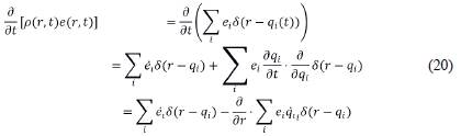
Where
and
where Φ ¡ is the internal energy of a particle defined as 1/2 mv i 2 + 1/2 Σ j Φ ij . Finally, by reorganizing it and using the definition of Π (r, t), we can express the energy density field as
For the mathematical details of the complete procedure, please refer to Evans & Morriss (2008) and Irving & Kirkwood (1950). An example can be found in the works of Camargo et al. (2018) and Camargo-Trillos (2017a) where a mesoscale model was derived from first principles and equations of hydrodynamics near a solid wall valid for the study of nanoscales.
The irreversible part (second term of Eq. 12)
The connection between the mesoscopic and macroscopic hydrodynamic equations is clearer if we simplify them. To express the second term of (12) we have to consider that everything happening at the microscale depends on external perturbations from the outside system, which can promote either a linear (close to thermal equilibrium) or non-linear (far from equilibrium) response. Here we try the linear response of the system before any external perturbation, which can be expressed in terms of the fluctuation properties of the system in thermal equilibrium and is the straightforward expression of the fluctuation-dissipation theorem (FDT) reflecting a general relationship between the response of a given system to an external disturbance and the internal fluctuation of the system in the absence of that disturbance. Thus, it is characterized by a response function linked to properties like admittance, impedance, etc. Moreover, internal fluctuation is characterized by a correlation function of the relevant physical quantities of a system fluctuating in thermal equilibrium equivalent to the fluctuation spectra. Therefore, perturbance promotes flux inside the system, and the coefficient (K jk ((α(t - s); s)) of Eq. (12) can be found by using Kubo relations at the mesoscale:

where α
j
(t) is a random variable receiving the information of the smallest scale in the form of random movement of particles. Subindices (j,k) are related to crossed phenomena, e.g., heat and electricity, etc. An example of, for example, mass transport can take K
jk
(α (t - s); s) as the diffusion coefficient (D (α (t - s); s)) and the force (F
k
(α (t - s))) will be the concentration gradient
 . Therefore, the random variable (α,- (t)) will be the random velocity of the Brownian particle (v(t)), and the flux
 will be the j-species mass flux like:

where
This is a way to connect the microworld and the macroworld. If the memory effect is not considered, the traditional constitutive equation of the flux (Fick, Newton, Fourier Ohm laws) is obtained:
Below, we show an example considering a response function of the type:

where is the microscopic time τ ≈ 10-12 - 10-14), characteristic of relaxation towards local equilibrium. Therefore:

If ∇φ varies slowly on the time scale ∼τ, one recovery Fick flow for the material transport is obtained:
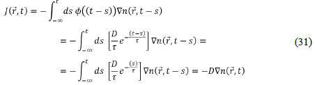
On the contrary, the kernel ϕ (t - s) or transport coefficient must be evaluated from molecular dynamics or an approximate expression such as
 .
.
An interesting case would be defining flux as a relevant variable (α
j
(t) = flux of energy). Therefore, in the case of heat transport,  would be the relevant variable, or
 .
The convective or mesoscopic part approximates the heat flux divided by the relaxation time
.
The convective or mesoscopic part approximates the heat flux divided by the relaxation time
 , which is the time the system takes in reaching the equilibrium state after it suffers the influence of a perturbation or the impact of an external force acting on the system. Finally, the diffusive part would be
 ; to arrive at the motion equation, the heat flux can be settled as:
By considering that there is no memory effect (Markovian approach), we get to the Cattaneo-Vernotte (Auriault, 2016) equation:
where τ is the relaxation time, k is the thermal conductivity, and ∇T is the temperature gradient. Up to this point, we have shown that the Navier-Stokes equations are derived from Eq. (12) for the isotropic system. Likewise, it can be extended to problems that require population balance on a smaller scale. Consequently, those equations of motion are simplified because the characteristic property of macroscopic variables varies slowly in time. It is possible to derive the set of hydrodynamic equations and derive from them others like mesoscale or macroscale.
This approach enables a fast jump from the microscale to the macroscale by implementing MC, EMD, and NEMD techniques to predict the transport coefficient of the Naiver-Stokes equation (diffusion, viscosity, conductivity, etc.) for physical analysis and update the microscopic information.
Example of heat diffusion with memory effects
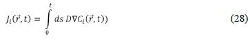
An example of memory effects can be seen in heat transfer processes. For example, for a one-dimensional domain of length L, the energy balance considering a heat flux by conduction following Eq. (31) is given by
where k is the thermal conductivity, k is the thermal conductivity at t = 0, C is the heat capacity, and p is the density. The parameters used in the simulation are ko = 1 W/(m - K), C = 1 J/(kg - K), p = 1 kg/m 3, L = 1 m. The first case to analyze is the heating of a flat plate with constant temperatures at x = 0 and x = L. In other words, Eq. (34) is subject to T = 100°C at x = 0; T = 25 °C at x = L, and T(x) = 25 °C at t = 0. Figure 4 shows the solution of Eq. (34) for three materials with different relaxation times (It is noted that the greater the relaxation time τ = 10-12 s, τ = 10 s, = 100 s). of the material, the longer it takes to reach a steady state. In this case, it clearly obeys a linear temperature profile.
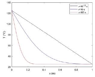
Since the expressions for the thermal conductivities of the three simulated materials are different (because they have different relaxation times), it would be expected that the steady-state behavior would also be different. However, in steady state (t → ∞) we have that
This equation implies that regardless of the relaxation time of the material, at a steady state, the thermal behavior -understood as the temperature profile and the heat flux- is the same. The previous analysis also indicates that the typical measurement method of thermal conductivity carried out in steady-state conditions would not always describe the thermal behavior of materials in a transient state adequately.
The importance of memory effects is also evidenced during pulsed heating processes where a transient thermal stimulus is applied to a material. To simulate this phenomenon, the following boundary conditions are used for Eq. (34)
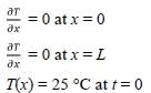
Additionally, a temperature pulse during 0.5 s generating a 100°C-increment at x = 0 is applied. Figure 5 shows the results of these simulations where the temperature evolution is presented in two locations (x = 0.1 m and x = 0.2 m) for three materials with different relaxation times.
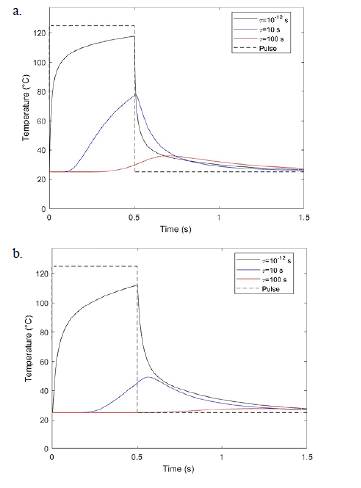
Figure 5 Temperature evolution of materials with different relaxation times in a heating system excited with a pulse at 5a) x = 0.1 m and 5b) x = 0.2 m
It is observed that as the relaxation time of the material increases, the "temperature signal" takes longer to arrive. For example, figure 5a shows that when t=100 s the temperature of the material continues to increase after the pulse has ended. Furthermore, figure 5b shows that the temperature of this same material starts increasing shortly after the pulse has ended. This behavior is known as "thermal lag" and has been observed in numerous experiments; although there is still no scientific consensus regarding its explanation, memory effects would allow a better understanding of this phenomenon.
Example of microhydrodynamic modeling at coarse-graining level on the mesoscale
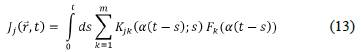
Camargo et al. (2018) and Camargo-Trillos (2017a) presented an example of a mesoscale model derived from the equations of hydrodynamics near a solid wall. In this model, the fluid moves according to a set of non-local hydrodynamic equations (hydrodynamic-level description) that explicitly include the solid and anisotropy forces of the system.
The model was built assuming a hydrodynamic level of mesoscale. The reversible contribution vj emerged from the free energy density functional accounting for impene trability whereas the irreversible contribution J j involved the velocity of both the fluid and the solid. The solid-fluid forces were localized in the vicinity of the solid surface, therefore, non-local hydrodynamic equations were required to consider the anisotropy in the fluid close to the solid and the interaction of forces with the solid, and non-local transport coefficient had to be estimated. Using the Marconian approach, the transport coefficients were explicitly expressed in terms of Green-Kubo formulae and estimated by the time correlation between microscopic variables.
Finally, dual basis functions δμ (r) and ψμ (r) constructed out of the finite-element basis function set Φμ (r) were implemented. The first one, δμ (r) discretized a continuum field of fluid velocity v
p
(r) by defining the discrete values at each node μ while the second basis function, ψμ (r) allowed us to construct a continuum field out of a discrete set of values
 (r) through interpolation (Camargo-Trillos, 2017b; Español & Donev, 2015; Torre et al.,
2019). As a result, a generalized dynamic density functional theory (DDFT) was developed by including the mass density field p(r, t) (as unusual approaches to DFT) and the momentum density g (r) of the fluid as relevant variables. Figure 6 shows a schematic summary of a mesoscopic model representing the hydrodynamics in nanopores.
(r) through interpolation (Camargo-Trillos, 2017b; Español & Donev, 2015; Torre et al.,
2019). As a result, a generalized dynamic density functional theory (DDFT) was developed by including the mass density field p(r, t) (as unusual approaches to DFT) and the momentum density g (r) of the fluid as relevant variables. Figure 6 shows a schematic summary of a mesoscopic model representing the hydrodynamics in nanopores.
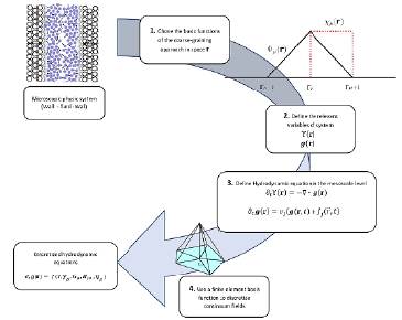
Figure 6 Mesoscopic model procedure for hydrodynamics in nanopores developed by Camargo et al (2018) and Camargo-Trillos (2017a).
The mesoscopic model was validated for a general hydrodynamic DDFT of simple fluids in the case of slit nanopores with planar flow configurations divided into n nodes (μ). In this simple geometry, only a reduced number of non-local transport coefficients (wall friction γμ, slip friction G μ , H μ , and viscous friction η μ ) are needed for the planar configuration (Figure 7a).
Figure 7 Validation of a mesoscopic model. a) Physical system in slit nanopores; b) momentum evolution of plug flow non-equilibrium molecular dynamics (dusted point) and mesoscopic model (line) taken from Camargo-Trillos (2017b)
The model at mesoscale allowed a close connection of the GC process and hydro-dynamic discretization of new relevant variables as v(r). In planar geometry, the continuum hydrodynamic equations for a fluid in a slit nanopore were discretized, thus allowing us to compute the Green-Kubo expressions explicitly for the non-local transport coefficients. Finally, it was possible to solve the continuum hydrodynamic of the mesoscale model numerically by a simple ODE function. Figure b compares the time evolution of a plug flow profile inside slit nanopores decaying to equilibrium for a mesoscopic model (line) and NEMD simulation (dusted point).
Remarks and conclusions
Based on these explanations, we can conclude that in the mathematical modeling of processes, each spatial scale has typical variables that describe it. The microscopic scale is characterized by the variables of position and velocity of each of the particles, which, if calculated, could perfectly describe the thermodynamics and transport phenomena typical of larger scales. However, calculating the position and velocity of a large number of N particles implies solving Newton's law for N times simultaneously, which may be an impossible task in terms of computational time.
On the other hand, if we start from a larger scale than the microscopic one, where we no longer talk about particles but about clusters that behave like individual particles, it is necessary to consider new variables such as the density of matter, energy, and charge. Now, if the spatial scale is further increased, phases can be differentiated and new variables known as effective properties, as well as the so-called transfer coefficients between phases, appear. Finally, non-local models applicable on the macroscopic scale, i.e., the thermodynamic scale, can arise from mesoscopic models integrating the equation of motion over the entire domain of real space to obtain an equation whose space-averaged relevant variables only vary with time.

