HYDROGEOLOGY

Spatio-temporal variability of groundwater depth in the Eghlid aquifer in southern Iran

Masoomeh Delbari^1*, Masoud Bahraini Motlagh² and Meysam Amiri³

¹ Associate Professor in the Department of Water Engineering, Faculty of Water and Soil, University of Zabol, Zabol, Iran, Tel: +98/542/2232113-8, Fax: +98/542/2255133, *Corresponding author Email: mas_delbari@yahoo.com

² Graduated M.Sc. Student of Water Resources Engineering, Department of Water Engineering, Faculty of Water and Soil, University of Zabol, Zabol, Iran

³ Scientific Staff in the Department of Water Resources, International Hamoun Wetland Research Institute, University of Zabol, Zabol, Iran

Manuscript received: 20/12/2012
Accepted for publication: 18/11/2013

ABSTRACT

Groundwater is the main water source for domestic and agricultural use in Eghlid, a city located in Fars province in southern Iran. Here, spatial and temporal changes in groundwater depth were monitored by using geostatistical methods at 41 observation wells in Eghlid during the wet and dry seasons of 1997, 2003 and 2010. Experimental semivariograms were calculated and modeled with the GS+ (Gamma Design Software, Plainwell, Michigan USA),and groundwater depth was interpolated by using the ordinary kriging (OK), simple kriging (SK) and inverse distance weighting (IDW) methods within the GIS environment. Moreover, groundwater depth fluctuations over 13 years (from 1997 to 2010) were calculated and mapped for wet and dry periods. The groundwater depth in the Eghlid aquifer exhibited a strong spatial correlation that followed a spherical model for three years. However, the spatial correlation distance was larger for both seasons in 1997 (greater than 27 km) than in 2003 (22 to 27 km) and 2010 (23 to 25 km). The cross-validation results indicated that OK resulted in the lowest root mean square error (RMSE) and mean error (ME) and was the most appropriate method for interpolating groundwater depth. Therefore, OK was used to map the spatial distribution of the groundwater depth over the study area. The resulting maps indicated that the spatial variability of groundwater depth was greater during the wet season than during the dry season over three years. In addition, changes in the depth to groundwater occurred more slowly during the wet seasons than during the dry seasons. Furthermore, the ground water depth decreased slightly from 1997 to 2003 and decreased considerably (2-13 m) from 2003 to 2010. Moreover, the decrease in the groundwater depth was more notable in the central to west and southern regions of the aquifer. Thus, these regions are critical and should be managed carefully to optimize groundwater resource exploitation.

Key words: Estimation, geostatistics, groundwater depth, spatial variation, GIS

RESUMEN

Las aguas subterráneas son la principal fuente hídrica para el uso doméstico y agrícola en Eghlid, una ciudad ubicada en la provincia de Fars, al sur de Irán. Aquí, los cambios temporales y espaciales en la profundidad de las aguas subterráneas se sondean a través de métodos geoestadísticos en 41 pozos de observación en Eghlid durante las estaciones de verano e invierno de 1997, 2003 y 2010. Se calcularon semivariogramas experimentales y se modelaron con el programa informático GS+, y la profundidad de las aguas subterráneas se interpolaron por el uso de krigging ordinario (OK), krigging simple (SK) y métodos de ponderación de distancia inversa (IDW) dentro del ambiente GIS. Sin embargo, la fluctuación de profundidad de las aguas subterráneas en cerca de 13 años (de 1997 a 2010) se calculó y se mapeó para las temporadas húmeda y seca. La profundidad de las aguas subterráneas en el acuífero de Eghlid muestra una fuerte correlación que sigue un modelo esférico de tres años. Sin embargo, la distancia de correlación espacial fue mayor para ambas temporadas en 1997 (mayor que 27 km.) y en 2003 (22 a 27 km.) y 2010 (23 a 25 km.). Los resultados de validación cruzada indicaron que el producto OK en la raíz cuadrada media de desviación más baja (RMSE) y Error Medio (EM) fueron los métodos más apropiados de interpolación de la profundidad de aguas subterráneas. Por lo tanto, el OK fue usado para mapear la distribución espacial de la profundidad de las aguas profundas en el área de estudio. El resultado de los mapas indican que la variabilidad espacial de la profundidad de aguas subterráneas fue mayor durante la temporada húmeda que durante la temporada seca en tres años. Adicionalmente, la profundidad de las aguas subterráneas fue menor durante la temporada húmeda que durante la temporada seca. Además, el nivel de las aguas profundas cedió ligeramente desde 1997 a 2003 y cayó considerablemente (de 2 a 13 metros). Además, el decrecimiento en el nivel de las aguas profundas fue más notable en las regiones de oeste, centro y sur del acuífero. Por ende, estas regiones son críticas y se deben manejar cuidadosamente para optimizar el recurso de explotación de las aguas subterráneas.

Palabras clave: Estimación; geoestadística; profundidad de aguas subterráneas; variación espacial; GIS.

Introduction

In Iran, which is located in an arid and semiarid region, surface water bodies are scarce. Consequently, groundwater is the main water source for domestic and irrigation purposes. Approximately 95 % of the fresh water resources in Iran are used for agricultural production, of which 80 % are obtained from groundwater (Ahmadi and Sedghamiz, 2008). Thus, groundwater resources are important for sustainable agriculture. In recent years, water table levels have dropped from 0.5 to 15 m beneath many agricultural lands, which has resulted in unproductive wells (Ahmadi and Sedghamiz, 2008). Therefore, to optimize groundwater resource exploitation, a detailed study regarding the spatial and temporal fluctuations of groundwater in this region is needed. In addition to water supply studies, knowledge regarding the spatio-temporal variability of groundwater depth is important for landfill characterization, management of agricultural salinity and chemical seepage (Buchanan and Triantafilis, 2009). However, the groundwater depth is generally measured at a small number of random locations. To obtain the required information on a dense grid, several interpolators should be employed. The common interpolation methods of classical statistics are not appropriate because they neglect the geographical positions of wells. In addition, it is well known that environmental variables are often spatially dependent. Geostatistics is a branch of statistics in which the spatial continuity behavior of the groundwater data is incorporated into the estimation process (Isaaks and Srivastava, 1989). Many researchers have mapped groundwater levels or optimized groundwater monitoring networks with geostatistical approaches (Delhomme, 1978; Sophocleous et al., 1982; Virdee and Kottegoda 1984; Tonkin and Larson, 2001; Nunes et al., 2004; and Delbari, 2013). Geostatistics can be used to improve the management and protection of water resources (Kumar and Sondhi, 2005; Reghunath et al., 2005). For example, Delbari (2013) compared several univariate and multivariate interpolation approaches for estimating groundwater levels in Iran. Kumar and Ahmad (2003) used geostatistical methods to estimate the groundwater depth in India. Furthermore, Desbarats et al. (2002) used a digital elevation model (DEM) to provide auxiliary data for estimating groundwater levels by using kriging with external drift. Cameron and Hunter (2002) determined an optimum sampling network by investigating the spatial and temporal variations of groundwater quality. In addition, Hu et al. (2005) investigated the spatial variability of groundwater levels, salinity and nitrate in northern China. These authors found that indicator kriging (IK) was more appropriate than ordinary kriging (OK) for mapping nitrate contamination risk. Kumar and Remadevi (2006) performed a spatial variability analysis of groundwater depth using data that were provided from more than 60 observation wells in India. These authors fit Spherical, Gaussian and exponential models to the experimental semivariograms and compared kriging estimates to inverse square distance (ISD) estimates. In this case, the kriging estimator with the Gaussian semivariogram model yielded the smallest error when estimating groundwater depth. Theodossiou and Latinopoulos (2007) used the kriging method to estimate groundwater levels and to optimize a groundwater-monitoring network. Furthermore, Ahmadi and Sedghamiz (2007, 2008) used geostatistics to map groundwater depth in Iran and Ta'any et al. (2009) investigated groundwater level fluctuations between 2001 and 2005 in the Amman Zarqa Basin in Jordan. These authors used OK to interpolate groundwater levels by using data from 31 wells. Sunet al.(2009) compared different methods for modeling groundwater level changes in 48 piezometric wells from 1981 to 2003 in China by using inverse distance weighting (IDW), radial basis function (RBF) and three kriging variants (the OK, simple kriging (SK) and universal kriging (UK) variants). These authors showed that the SK method was the most appropriate method among those tested.

This study aimed to investigate the spatial and temporal changes of the groundwater depth in an aquifer near Eghlid city, which is located in Fars province in southern Iran. Groundwater depth data were collected during dry and wet seasons in1997, 2003 and 2010. The OK, SK and IDW methods were used.

Methodology

Study area and groundwater depth

The city of Eghlid is located in Fars province in southern Iran, covers an area of 7054 sq. km and is located at 31° 13' N latitude and 52° 55' E longitude. Eghlid is allocated in a mountainous and highland region. The city of Eghlid follows the Zagross Mountains and Bell Mountains to the south with a maximum elevation of 3943 m asl. This area is characterized by cold winters and mild summers with minimum and maximum temperatures of -22 and 37 °C, respectively. The average annual rainfall levels in the city and highland villages are 300-330 mm and 400-600 mm, respectively. The study area includes an aquifer that covers an area of approximately 716.2 sq. km (Figure 1). The elevation in this region fluctuates from 2068 m west of the aquifer to 2690 m southeast of the aquifer. However, several small regions northwest of the study area are characterized by high elevation. Furthermore, Eghlid is an important location for agricultural production, especially for wheat, barley, potato and fruit production (including grapes, walnuts, apples and pears).

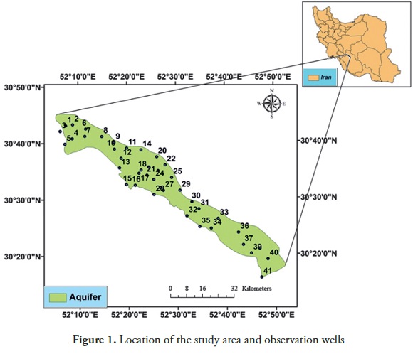
Groundwater resources provide an important water source for drinking water and water for agricultural purposes. Here, the spatiotemporal variability of the groundwater depth was determined by using data from 41 observation wells that were placed throughout the study area. The geographical locations of the wells are shown in Figure 1. For these observation wells, the monthly averages of groundwater depth data for March (wet season) and September (dry season) were monitored between 1997 and 2010.These data were used for the geostatistical analysis. To consider temporal fluctuations, data were analyzed from 1997, 2003 and 2010.

Geostatistics

The theory of geostatistics has been expressed in many textbooks, including those of Isaaks and Srivastava (1989) and Goovaerts (1997). Here, a brief description of the geostatistical methodsthat were used in this study is presented. In geostatistics, a semivariogram is used to quantify the differences between sampled data values as a function of their separation distance, h. In practice, the experimental semivariogram, *(h), is calculated as follows:

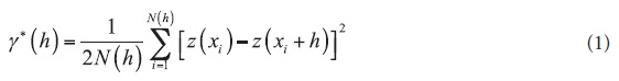
where N(h) is the number of sample pairs that are separated by a vector h, and z(x_i) and z(x_i+h) are the values of the variable z at locations of x_i and x_i+h, respectively. However, for kriging analysis, an appropriate theoretical model should be used to fit the experimental data. The most widely used models include the spherical, exponential and Gaussian models. The spherical model used in this study is defined as follows:

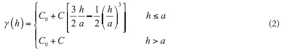
where C₀ is the y-axis intercept (the "nugget effect"), C₀+C is the "sill", which is near the sample variance, and a represents the range of influence.

Ordinary kriging

OK assumes that the mean is stationary but unknown. In addition, the OK estimator is known as the best linear unbiased estimator (BLUE) and is defined as follows (Journel and Huijbregts, 1978):

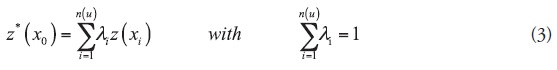
where z*(x₀) is the OK estimator at location x₀, z(x_i) is the observed value of the variable at location x_i, λ_i is the weight assigned to the known values near the location to be estimated and n(u) is the number of neighboring observations. The values of λ_i are weighted to obtain a sum of unity, and the error variance is minimized as follows:

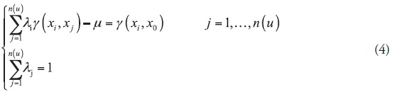
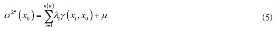
where μ is the Lagrange coefficient for minimizing the OK estimation variance, γ(x_i, x_j) is the average semivariogram value between the observed values and γ(x_i, x₀) represents the average semivariogram value between the location x_i and the location to be estimated (i.e., x₀).

The OK estimation variance (or standard deviation) can be used as a measure of the estimation uncertainty as follows:

Simple kriging

For example, OK and SK assume a stationary but known mean. In addition, OK uses local averages and SK uses entire observation averages. The SK estimator is given as follows:

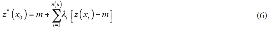
where m is the mean value of the variable z and λ_i is the weight assigned to the residual value of z(x_i) from the mean. This estimate is unbiased because E [z(x_i)-m]=0 and E [z*(x₀)]=m=E [z(x₀)].

Inverse distance weighting

When using IDW, the unknown value at location x₀, z^*(x₀) is estimated from the linear weighted average of several neighboring observations as follows:

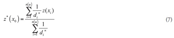
where z(x_i) is the observed value at location x_i, d_i is the distance between the interpolated and observed values and a is an exponent. In IDW, the weights are inversely proportional to a power of the distance between the observations and the location x_0. As the value of power aincreases, the effect of the farthest observations on the estimated value decreases. In Here, values of a were set to 1, 2 and 3.

Comparison of the interpolation methods

Here, the cross-validation technique (Isaaks and Srivastava 1989) was used to compare different interpolation approaches. The evaluation criteria that were used included the root mean square error (RMSE) and the mean error (ME), which are defined as follows:

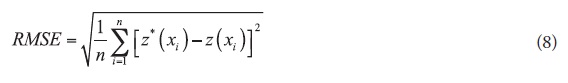
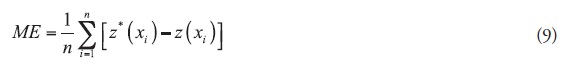
where z^*(x_i) and z(x_i) are the estimated and measured values at location x_i, respectively, and n is the number of observations. The most appropriate method has the smallest RMSE. In addition, the best estimator has an ME near zero.

Here, the semivariogram calculations and groundwater depth modeling were performed in GS+ (Robertson, 2000). Interpolation and mapping were performed by using the ArcGIS Geostatistical Analyst.

Results and Discussion

Statistical Analyses

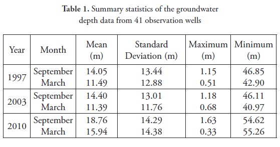
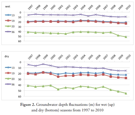
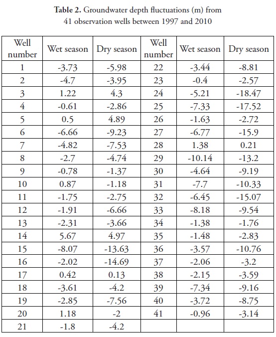
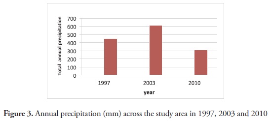
A summary of the groundwater depth data is presented in Table 1. The mean groundwater depth in 2010 was greater than its corresponding value in 1997 and 2003. In contrast, the groundwater depth did not fluctuate much between the two seasons between 1997 and2003. However, the groundwater depth significantly decreased (approximately 4.5 m) between 2003 and 2010. The groundwater depth fluctuations of four randomly selected wells (wells number 13, 19, 29, and 36) during the dry (September) and wet (March) seasons of 1997 and 2010 are shown in Figure 2. The groundwater depth fluctuations were minimal until 2006 (for wet season) and 2007 (for dry season) (Figure 2). However, the groundwater depth significantly decreased after 2007. The increases and decreases in groundwater depth for all 41 wells between 1997 and 2010 are presented in Table 2. In September, the largest decrease occurred at well number 24 (18.47 m).In March, the largest decrease (10.14 m) occurred at well number 29. Both of these wells are located near the center of the study area (Figure 1). As shown in Table 2, in majority of wells, the drop in March was less than the drop in September, which could be attributed to changes in aquifer storage. Recharge generally occurs in the late winter and spring seasons, when precipitation is generally the greatest and the evapotranspiration rate is low. In Figure 3, the amounts of annual rainfall during 1997, 2003 and 2010 are shown. A drastic reduction in rainfall occurred between 2003 and 2010. This decrease potentially resulted in the deeper groundwater depth between 2003 and 2010.

Table 3.

Geostatistical Analyses

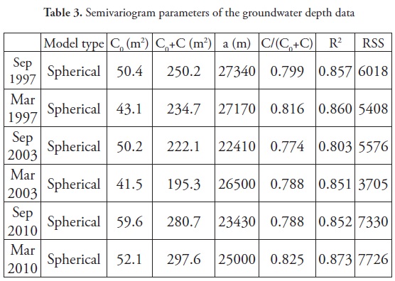
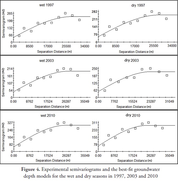
To investigate the spatial autocorrelations of the groundwater depth for selected years, the omnidirectional experimental semivariogram was calculated (Figure 4). The best theoretical model of the semivariogram is shown in Figure 4. To determine the directional behavior of the spatial variability of the groundwater depth, the experimental semivariogram of groundwater depth was calculated for four directions (0, 45, 90 and 135 degrees) with an angle tolerance of 22.5°.These results did not show any significance differences. Thus, the groundwater depth was assumed as isotropic and the semivariograms shown in Figure 4 were considered for further analysis. The groundwater depth during the wet and dry seasons in 1997, 2003 and 2010 was strongly spatially correlated because the ratio of the nugget effect to the sill of the semivariograms was small (Figure 4). The spatial structure of the groundwater depth during the wet and dry seasons in 1997, 2003 and 2010 followed a spherical model. Similarly, Kumar and Ahmad (2003) indicated that the spherical model was the best for modeling the spatial structure of groundwater depth. However, Delbari et al. (2010) and Ahmadi and Sedghamiz (2007) indicated that the spherical and exponential models were the best theoretical semivariogram models. Ta'any at el. (2009) and Kumar and Remadevi (2006) introduced the Gaussian model and Mendes and Lorandi (2008) introduced the exponential model as the best fitted semivariogram models for predicting groundwater levels. As shown in Table 4, the smallest and largest nugget effects (random variance) were found for groundwater depths in March 2003 and September 2010, respectively. The influence range was greatest (approximately 27 km) during September 1997 and smallest (approximately 22 km) during September 2003.

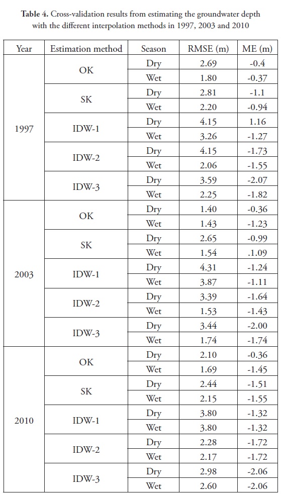
For the interpolation of groundwater depth, the OK, SK and IDW methods were used with exponents of 1, 2 and 3. The RMSE and ME values that were associated with each method were calculated through cross-validation and are presented in Table 4 for 1997, 2003 and 2010. These results indicated that the OK approach is the most appropriate interpolation approach for estimating groundwater depth because it yielded the lowest RMSE for all three years and all seasons and resulted in the smallest bias (ME) in most cases. The IDW method, which does not consider the spatial correlation of the observations during the estimation processes, often resulted in the highest error. In the study by Kumar and Remadevi (2006), OK was more accurate than IDW for groundwater level interpolation.

Figure 5 shows the maps of interpolated groundwater depth during the wet and dry seasons of 1997, 2003 and 2010 that were obtained by OK. Greater spatial variability occurred for the groundwater depth during the wet seasons than during the dry seasons. This finding potentially resulted from the spatial variations of the groundwater recharge and discharge. The groundwater depth was greater from the center to the west of the aquifer, which potentially resulted from the lower topographical elevation and greater groundwater resource exploitation. A drastic decrease in groundwater depth occurred between 1997 and 2010 throughout the study area. This decrease resulted from the excessive exploitation of groundwater resources for drinking and agricultural purposes and from the lack of precipitation during the most recent years. Moreover, as shown in Figure 5, the groundwater depth significantly increased between March and September each year. For example, in March 2010, the groundwater depths in many areas in the southern, southeastern and upper portions of the study area were approximately 2 m below the surface. However, in September these groundwater depths increased from 2 to 8 m. This change resulted from increasing water levels during the late winter and spring and decreasing water levels through the summer and fall.

Figure 5.

As previously indicated, the estimated standard error of OK can be used to measure the uncertainty of groundwater depth estimates. The maps of the OK estimation error (Figure 6) show that a smaller uncertainty occurs near the observation wells (i.e., the upper half (except northwest) and southeastern regions of the study area). Larger uncertainty regarding groundwater depth estimates can be observed in regions where more variability in the spatial distribution of groundwater depths (e.g., northwest) occurs and where the sample points are farther apart (e.g., near the center of the study area). In addition, larger uncertainty can be observed around the borders of the study area, especially in the lower half, which has no observation wells. These locations are primary candidates for digging additional wells in the future.

Figure 6.

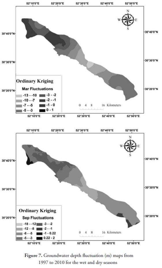
In addition, groundwater depth fluctuation maps were obtained from 1997 to 2010 during the wet and dry seasons (Figure 7). During the wet season, the groundwater depth decreased by7 to 10 m in the central regions of the study area and by 3 to 5 m in the southern regions of the study area. During the dry season, the groundwater depth decreased by approximately 8 to12 m in the central regions of the study area and by 5 to8 m in the southern regions of the study area. This significant decrease in groundwater level potentially resulted from (1) lower rainfall during recent years and from (2) high groundwater resource exploitation. Overall, these results could be used in future macro- policies, e.g., using modern irrigation systems rather than conventional irrigation methods or enhancing the efficiency of current irrigation systems.

Conclusions

Here, the spatiotemporal variability of groundwater depth was investigated. Three interpolation methods, including OK, SK and IDW, were applied to estimate the groundwater depth throughout the study area. The groundwater depth is strongly spatially correlated and its spatial structure follows a spherical model. The OK method was the most appropriate method for the three investigated years. The spatial distribution maps of groundwater depth showed that groundwater depth in Eghlid aquifer did not change much between 1997and 2003, but decreased in 2010. This decrease potentially resulted from the lower annual rainfall in 2010 relative to 2003. Moreover, the generated maps clearly indicated that the groundwater depth decreased during the wet seasons relative to the dry seasons. The groundwater depth fluctuations maps indicated that the groundwater decrease was more noticeable in the central and southern regions of the aquifer than in the northern regions, which potentially resulted from the higher density of observation wells in the central and southern regions of the aquifer. Therefore, for sustainable exploitation of groundwater resources, these regions should be carefully managed. Potential management options include the use of modern irrigation techniques and changing cropping patterns to crops that require less irrigation.

Moreover, unlike inverse distance weighting, ordinary kriging can be used to produce maps of the estimation errors that are associated with the groundwater depth estimates. These maps can be used to identify the next locations for new monitoring wells.

Acknowledgements

The authors would like to thank the anonymous reviewers for their useful comments that helped improve this manuscript.

References

Ahmadi, S.H. and Sedghamiz, A. (2007) Geostatistical analysis of spatial and temporalvariations of groundwater level. Environ. Monit. And Assess., 129, 277–294.         [ Links ]

Ahmadi, S.H. and Sedghamiz, A. (2008) Application and evaluation of kriging and cokriging methods on groundwater depth mapping. Environ Monit Assess., 138, 357–368.         [ Links ]

Cameron, K. and Hunter, P. (2002) Using spatial models and kriging techniques to optimize long-term ground-water monitoring networks: A case study. Environmetrics, 13, 629–656.         [ Links ]

Delbari. (2013). Accounting for exhaustive secondary data into the mapping of water table elevation. Arab J Geosci. In press, DOI 10.1007/s12517-013-0986-2.         [ Links ]

Delbari, M., Afrasiab, P. and Miremadi, S.R. (2010) Spatio-temporal variability analysis of groundwater salinity and depth (Case study: Mazandaran province). Irrigation and drainage Journal, 3 (4), 359–374 (in Persian).         [ Links ]

Delhomme, J.P. (1978). Kriging in hydrosciences. Adv. Wat. Resour., 1, 251–266.         [ Links ]

Desbarats, A.J., Logan, C.E., Hinton, M.L. and Sharpe, D.R. (2002) On the kriging of water table elevations using collateral information from a digital elevation model. Journal of Hydrology, 255, 25–38.         [ Links ]

Fayzieva,D., Kamilova, E. and Nurtaev, B. (2008) On Development of GIS-Based Drinking Water Quality Assessment Tool for the Aral Sea Area. J.E. Moerlins et al. (eds). Published by: Springer Netherlands, Transboundary Water Resources: A Foundation for Regional Stability in Central Asia, 183–192.         [ Links ]

Goovaerts, P. (1997) Geostatistics for Natural Resources Evaluation. New York: Oxford University Press.         [ Links ]

Hu, K., Huang, Y., Li, H., Li, B., Chen, D. and White, R. E. (2005) Spatial variability of shallow groundwater level, electrical conductivity and nitrate concentration, and risk assessment of nitrate contamination in North China Plain. Environment international, Vol. 31 (6), 896–903.         [ Links ]

Isaaks, E.H. and Srivastava, R.M. (1989)" An Introduction to Applied Geostatistics". New York: Oxford University Press, 561pp.         [ Links ]

Journel, A.G. and Huijbregts, C.J. (1978) Mining Geostatistics. London Academic Press, New York, 600 p.         [ Links ]

Kumar V. and Remadevi. (2006) Kriging of Groundwater Levels – A Case Study. Journal of Spatial Hydrology,6(1):81–94.         [ Links ]

Kumar, D. and Ahmed, Sh. (2003) Seasonal behavior of spatial variability of groundwater level in a granitic aquifer in monsoon climate. Current Science, 84(2), 188–196.         [ Links ]

Leuangthong, O., McLennan, J.A. and Deutsch, C.V. (2004) Minimum acceptance criteria for geostatistical realizations. Natural Resources Research, 13, 131–141.         [ Links ]

Li, L. and Revesz, P. (2004) Interpolation methods for spatio temporal geographic data. Computers, Environment and Urban Systems, 28, 201–227.         [ Links ]

Mendes, R.M. and Lorandi, R. (2008) Analysis of spatial variability of SPT penetration resistance in collapsible soils considering water table depth. Engineering Geology, 101, 218–225.         [ Links ]

Nunes, L.M., Cunha, M.C. and Ribeiro, L. (2004) Ground water monitoring network optimization with redundancy reduction. Journal of Water Resources Planning and Management, 130, 33–43.         [ Links ]

Patriarche, D., Castro, M.C. and Goovaerts, P. (2005) Estimating regional hydraulic conductivity fields A comparative study of geostatistical methods. Mathematical Geology, 37, 587–613.         [ Links ]

Reghunath, R., Sreedhara Murthy, T.R. and Raghavan, B.R. (2005) Time series analysis to monitor and assess water resources: A moving average approach. Environmental Monitoring and Assessment, 109, 65–72.         [ Links ]

Robertson G.P. (2000) 'GS+: Geostatistics for the environment sciences. GS+ User´s Guide Version 5: Plainwell, Gamma design software, 200 p.         [ Links ]

Rouhani, Sh. and Wackernagel, H. (1990) Multivariate geostatistical approach to space-time data analysis. Water Resources Research, 26, 585–591.         [ Links ]

Sophocleous, M., Paschetto, J.E. and Olea, R.A. (1982) Groundwater network design for northwest Kansas, using the theory of regionalized variables. Groundwater, 20, 48–58.         [ Links ]

Sun, Y., Kang, Sh., Li, F. and Zhang, L. (2009) Comparison of interpolation methods for depth to groundwater and its temporal and spatial variations in the Minqin oasis of northwest China. Environmental Modelling and Software 24, 1163–1170.         [ Links ]

Ta'any, R.A., Tahboub, A.B. and Saffarini, G.A. (2009) Geostatistical analysis of spatiotemporal variability of groundwater level fluctuations in Amman–Zarqa basin, Jordan: a case study. Environ. Geol., 57, 525–535.         [ Links ]

Theodossiou, N. and Latinopoulos, P. (2006) Evaluation and optimization of groundwater observation networks using the Kriging methodology. Environmental Modeling and Software 21, 991–1000.         [ Links ]

Tonkin, M.J. and Larson, S.P. (2001) Kriging water levels with a regional-linear and point-logarithmic drift. Ground Water, 40, 185–193.         [ Links ]

Virdee, T.S. and Kottegoda, N.T. (1984) A brief review of kriging and its application to optimal interpolation and observation well selection. Hydrol. Sci. J., 29, 367–387.         [ Links ]

Yidana, S.M., Ophori, D. and Yakubo, B.B. (2008) Groundwater Quality Evaluation for Productive Uses— The Afram Plains Area, Ghana. J. Irrig. and Drain. Engrg., 134(2), 222–22        [ Links ]