1. Introduction

Remote sensing can be understood as a technique responsible for identifying, measuring and analyzing objects on the Earth's surface without direct contact, using sensors installed on satellites, aircraft or drones, which record electromagnetic radiation reflected or emitted by surfaces (^{Alam, 2019};^{Awange & Kiema, 2019}; ^{Fu, Ma, Chen & Chen, 2020}; ^{Thakur et al., 2017}; ^{Torres, Valdelamar & Saba, 2023}). These sensors capture information across various bands of the electromagnetic spectrum, enabling discrimination between object types (^{Navalgund, Jayaraman & Roy, 2007}). Compared to traditional data collection, remote sensing is non-invasive, faster, and more efficient, enabling large-scale and real-time monitoring even in inaccessible areas (^{Abdulraheem et al., 2023}; ^{Lechner, Foody & Boyd, 2020}). This makes it highly suitable for observing environmental changes such as soil degradation, crop monitoring, and deforestation.

Among remote sensing techniques, hyperspectral imaging stands out for combining digital imaging and spectroscopy, capturing hundreds of narrow and contiguous spectral bands that enable the identification of materials through their unique spectral signatures (^{Datta et al., 2022}; ^{Grewal, Kasana & Kasana, 2023}). These images form data cubes (x, y, λ), with each pixel containing a full reflectance spectrum (^{Fei, 2019}; ^{Lu & Fei, 2014}), allowing detailed material classification. However, hyperspectral images pose challenges due to their high dimensionality, requiring methods that are not only effective but also computationally efficient (^{Chang et al., 2022}; ^{Hu, Wang, Jiang, Zhang & Ma, 2024}; ^{Plaza et al., 2009}).

Given the high computational cost of deep learning methods such as 3D-CNNs, and the redundancy of hyperspectral data, this article proposes the evaluation of two computational approaches for water body detection in hyperspectral images from the city of Cartagena, Colombia: the Spectral Differential Similarity (SDS) method and a sequential neural network (ANN). A dataset of 200 spectral signatures was used to fit both models, which were later deployed on a hyperspectral image of 380 bands and 725x850 pixels.

The rest of the article is organized as follows: The section two mentioned previous studies on the use of hyperspectral images for environmental monitoring, detection of water bodies, and microplastics; section three presents the methodological phases that guided the study. Then, the results are discussed, including the adjustment and evaluation of both methods, their application to the full image, and the computational performance analysis. Finally, conclusions and future directions are provided.

2. Background

Hyperspectral imaging has been extensively used in environmental monitoring due to its capacity to detect subtle differences in material composition through spectral signatures. For instance, studies such as ^{Kim et al. (2020)}, ^{Niu, Tan, Wang, Du & Pan (2024)}, and ^{Waczak et al. (2024)} used hyperspectral and satellite imagery to map water bodies and analyze parameters like chlorophyll-a concentration and water quality. Similarly, works by ^{Huang et al. (2021)}, ^{Prosek et al. (2020)}, and ^{Shan et al. (2019)} applied machine learning algorithms -such as SVM, neural networks, and linear discriminant analysis- for water body identification and contaminant detection with high precision.

Further research has addressed more specific environmental threats, such as microplastics. ^{Ali, Lyu, Ersan & Xiao. (2024)}, ^{Piarulli et al. (2022)}, and ^{Serranti, Palmieri, Bonifazi & Cózar (2018)} employed hyperspectral imaging combined with machine learning to detect and classify plastic particles in oceans, freshwater bodies, and soil. Techniques such as dark-field microscopy (^{Fakhrullin, Nigamatzyanova & Fakhrullina, 2021}) and laser-induced fluorescence (^{Mahmoud & El-Sharkawy, 2024}) have also been integrated with hyperspectral imaging for identifying pollutants in complex environments.

Despite the proven efficacy of these approaches, hyperspectral data processing remains a challenge due to the large volume of redundant spectral information. Deep learning techniques like 3D-CNNs, while accurate, are computationally intensive and less suitable for real-time applications. This has led researchers to explore dimensionality reduction techniques such as principal component analysis (PCA) and more efficient computational models (^{Plaza et al., 2009}; ^{Wang, Hu, Jiang & Ma, 2022}).

This body of literature highlights the need for methods that strike a balance between accuracy and computational efficiency, especially for real-time environmental monitoring tasks like water body detection.

3. Methodology

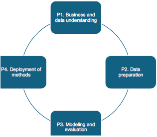
For the development of the present research, an adaptation of the CRISP-DM data mining methodology was made to four phases: P1. Business and data understanding, P2. Data preparation, P3. Modeling and evaluation, and P4. Method deployment (see Figure 1). The CRISP-DM methodology was chosen taking into account that it is independent of the technological sector, highly customizable and provides a clear and repeatable structure for data mining and machine learning projects, facilitating planning, communication and documentation in experienced teams and those with less technical experience (^{Kolyshkina & Simoff, 2021}; ^{Schröer, Kruse & Gómezc, 2021} ; ^{Shimaoka, Ferreira & Goldman, 2024}).

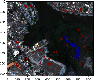
In phase 1 of the methodology, a total of 200 sample spectral signatures were selected from a hyperspectral image of the Manga neighborhood in the city of Cartagena with 725x850 pixels and 380 reflectance bands, in such a way that 100 signatures correspond to water bodies and 100 signatures belong to other materials such as: vegetation, roads, cement roofs, metal roofs, containers, etc. The number of spectral signatures selected (100 and 200) was determined through preliminary tests aimed at identifying a balance between the spectral representativeness of the classes and the computational stability of the model. In initial trials, subsets of different sizes (50, 100, 200, and 300 signatures) were evaluated, and it was observed that intra-class variability stabilized at 100 signatures and that an increase above 200 did not significantly improve accuracy, but instead increased computational cost. Therefore, 100 and 200 signatures were adopted as representative thresholds for the comparative analysis.

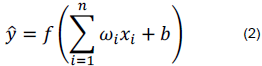
These signatures served for the adjustment and evaluation of the identification capacity of the spectral signature of freshwater bodies by each of the considered methods. These 200 pixels or spectral signatures were selected by visual inspection and are presented in Figure 2, in which the 100 sample pixels of water bodies are shown in blue and the 100 pixels corresponding to other materials in red. These signatures were queried through the use of the spectral library, which allows obtaining the information of the reflectance bands as a numpy array of 380 positions.

Note: Own elaboration

Figure 1 Methodology considered 

Note: Own elaboration

Figure 2 Sample pixels selected from water bodies and other materials 

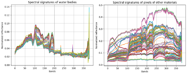
In this same regard, Figure 3 shows the 100 normalized spectral signatures associated with water body pixels and the 100 normalized signatures corresponding to pixels of other materials, in such a way that it can be appreciated that it can be appreciated how the spectral signatures of water bodies have a set of characteristic peaks along the spectrum that provide the methods with the possibility of differentiating them from other materials.

Note: Own elaboration

Figure 3 Sample spectral signatures of water bodies and other materials 

Now then, in phase 2 of the methodology, the characteristic pixel or average pixel band by band was obtained for the SDE method from the 100 spectral signatures of water bodies, while for the artificial neural networks model a dataset was formed with the 200 sample spectral signatures adding a label 1 for water body pixels and a label 0 for pixels of other materials (see Figure 4). The characteristic spectral signature was calculated through the use of array operations and was used by the SDS method to calculate the similarity with the two groups of spectral signatures and identify the detection thresholds. Data processing and analysis were performed in Python 3.10, using specialized libraries such as NumPy, Pandas, Matplotlib, TensorFlow, and Scikit-learn. Additionally, the Orange 3.34 environment was used for visual data analysis, cross-validation of models, and the generation of modular experimental flows. The integration of Python and Orange allowed us to combine the flexibility of programming with the graphical interpretation of results, improving the traceability of the classification process. Likewise, the dataset of 200 signatures was used to perform the adjustment and evaluation of the ANN model, in order to obtain performance metrics. It is possible to appreciate from Figure 4 how the columns of the dataset correspond to the reflectance bands, while the predictor attribute is binary and corresponds to the type of pixel to be classified.

Note: Own elaboration

Figure 4 Dataset composed of spectral signatures 

Likewise, in phase 3 of the methodology, the two proposed methods were implemented, adjusted and evaluated with the dataset of 200 spectral signatures. Thus, with regard to the SDS method, the characteristic spectral signature was used and the similarity based on the difference of the 380 was calculated with the two groups of sample pixels obtaining for each case the minimum and maximum percentage similarity, in such a way that it was verified that the minimum similarity with the group of water body pixels is greater than the maximum similarity obtained with pixels of other materials, since otherwise it is necessary to select the most relevant bands of the image where no overlap occurs. Based on the above, the minimum percentage similarity obtained with water body pixels is taken as the detection threshold. For the case of the sequential ANN model, the model was structured with different hidden layer configurations and its performance was evaluated at 100 epochs identifying the behavior of the accuracy metric or accuracy percentage in both the training set (80%) and the test set (20%), choosing the model with better stability and highest accuracy percentage. The architecture structuring was performed using the TensorFlow library considering 380 inputs corresponding to the spectral bands, a variable set of densely connected hidden layers, and a binary output. The ReLU activation function was implemented after each hidden layer to introduce non-linearity, while the sigmoid function was used in the output layer to obtain classification probabilities. The model architecture was defined using TensorFlow's Sequential class, incorporating regularization through Dropout in each hidden layer to prevent overfitting. Training was performed using the Adam optimizer with a learning rate of 0.001 and the binary_crossentropy loss function, appropriate for the binary nature of the classification problem. The ADAM (Adaptive Moment Estimation) optimizer was used for the training process. ADAM is widely used in deep learning due to its stability and efficiency in high-dimensional problems. ADAM combines the advantages of the AdaGrad and RMSProp methods, dynamically adjusting the learning rates for each parameter, which improves convergence and prevents oscillations in the gradient. Its adoption in this study was based on its reported effectiveness in previous research applied to hyperspectral images (^{Chang et al., 2022}; ^{Ali et al., 2024}) and its compatibility with compact neural network architectures (^{Datta et al., 2022}).

The spectral differential similarity (SDS) method is based on the calculation of the summation of the absolute value of the differences between the characteristic pixel X and the unknown pixel or spectral signature Y, as expressed in equation (1), where X _i and Y _i represent the reflectance values of the spectral signatures X and Y in spectral band I (^{Chen et al., 2025}). In this way, the closer to 0 the summation of the differences between spectral signatures X and Y is, the spectral signatures tend to be more similar and the SDS value approaches 100%.

On the other hand, with regard to the ANN model, the implementation of its architecture through the TensorFlow library can be mathematically modeled through equation (2):

Where x _i represents the neuron inputs,ω_i, the weights associated with each input, b is the bias, f is the activation function (such as ReLU, tanh, sigmoid) and is the estimated output of the neuron.

Finally, in phase 4 of the methodology, we proceeded with the deployment of the two methods adjusted in the previous phase on the complete hyperspectral image of the Manga neighborhood in the city of Cartagena, obtaining in each case and comparing the percentage of detected water body pixels. Likewise, the two methods are evaluated in 25, 50, 75 and 100 repetitions on a region of the reference image of 50x50 pixels and 380 bands, in order to obtain the average processing time per repetition and the total average processing time, in order to determine the relative computational efficiency. A small region of the reference hyperspectral image was chosen to perform the multiple repetitions of the computational methods in order to more easily obtain the response times and avoid overloads in RAM memory consumption, in such a way that this approach allows evaluating the algorithm performance in a controlled manner while maintaining the spectral representativeness of the data, since the computational characteristics scale proportionally with the image size.

4. Results

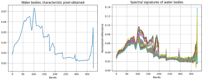
Regarding the results obtained in this research, in the first instance we proceeded with the determination of the average pixel or characteristic spectral signature of water bodies from the set of 100 pixels or sample spectral signatures of water bodies. This signature was calculated from Python's numpy library through the band-by-band average across the total of 380 reflectance bands and is presented in Figure 5, along with the 100 sample pixels. It should be mentioned that this characteristic spectral signature was used to compare the 200 sample signatures and determine the minimum detection threshold from which the SDS method begins to detect pixels or signatures of water bodies. The sample was duplicated in order to increase the spectral diversity of the training data and reduce possible biases of underrepresentation in minority classes. This strategy made it possible to stabilize the accuracy indicators and improve the generalization of the model without altering the original distribution of the signatures.

Note: Own elaboration

Figure 5 Characteristic spectral signature of water bodies 

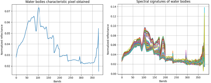
Now then, when applying the SDS method operating the characteristic spectral signature or average pixel with the two groups of average pixels, the minimum and maximum percentage similarity was obtained for each group of sample pixels, in such a way that Figure 6 shows the minimum similarity percentage with water body pixels and the maximum similarity percentage with pixels of other materials.

Note: Own elaboration

Figure 6 Minimum and maximum percentage similarity 

From the evaluation of the SDS method with the 200 sample pixels, it was obtained that the minimum percentage similarity with water body pixels exceeds by 0.003% the maximum similarity with pixels of other materials, which indicates that although the difference is narrow, no overlap occurs and the SDS method can detect spectral signatures of water bodies if the percentage similarity between a determined pixel of the image and the characteristic spectral signature is superior to 99.991%. According to the above, we proceeded with the deployment of the SDS method on the complete reference image of the Manga neighborhood, taking as reference the minimum detected threshold.

Thus, Figure 7 presents both the implementation of the method on the entire image, as well as the detected zones on an RGB representation of the hyperspectral image.

Note: Own elaboration

Figure 7 Deployment of the SDS method on the reference hyperspectral image 

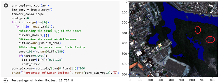
In Figure 7 it can be appreciated how the method performs the iteration for each pixel i, j of the image, after which the summation of the absolute value of the difference between said pixel and the characteristic spectral signature of water bodies is obtained, to subsequently determine the percentage of spectral differential similarity. After the above, it is verified if the percentage similarity is greater than the threshold of 99.991 and in case this condition is met, the counter of water body pixels is incremented and the evaluated pixel is painted blue. Thus, as a result of the method deployment, it is obtained that 13.734% correspond to water body pixels. In general terms, it can be appreciated how the method continuously detects water pixels in correct zones, however it makes some small errors classifying some vegetation zones as water pixels.

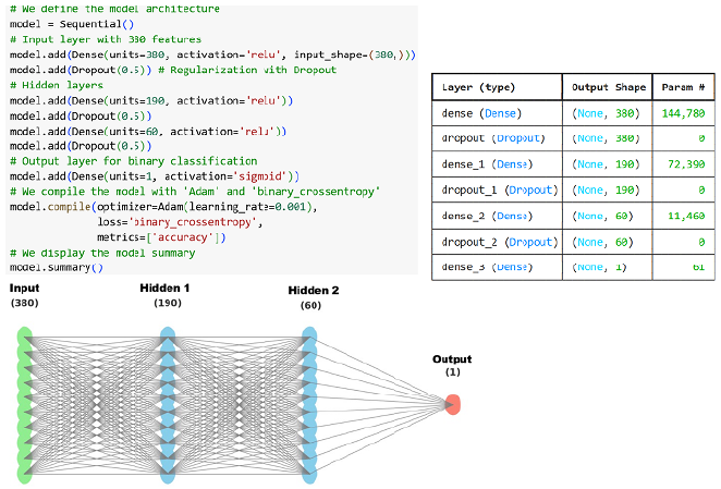
Regarding to the structuring of the sequential ANN neural architecture, different hidden layer configurations were evaluated, identifying that the configuration that has a better fit is that of the model with 380 inputs (considering the 380 columns of the dataset), 2 hidden layers (190 and 60 neurons) and an output layer taking into account the binary nature of the classification problem. It should be mentioned that after each hidden layer the ReLU activation function was implemented, while for the final layer a sigmoid activation function was employed.

Figure 8 shows both the model summary generated by TensorFlow and its corresponding architecture.

Note: Own elaboration

Figure 8 Architecture of the ANN model 

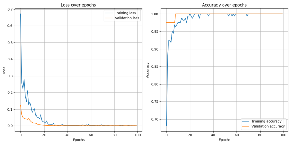
Once established the ANN neural network architecture, the training and validation of the model was performed during 100 epochs using a batch size of 32, employing the training and test sets distributed in proportions of 80% and 20% respectively. According to these parameters, Figure 9 shows the evaluation of the model performance in terms of loss and accuracy through the analyzed epochs.

Note: Own elaboration

Figure 9 Model performance assessment and loss function analysis across training epochs 

The results of Figure 9 clearly show how the model improves in both the loss function and accuracy as training progresses. Regarding the loss behavior, it is notable that the training loss drops rapidly in the first 20 epochs and then remains stable at low levels. For its part, the validation loss also descends markedly at the beginning, but it is interesting to observe that around epoch 30th both curves begin to converge, showing a much smaller gap between them, which indicates a better balance in learning. In the case of the accuracy metric, the behavior is equally adequate. In this way, the training accuracy rises in an accelerated manner in the first epochs and achieves values close to 1.0 around epoch 20. The validation accuracy follows a similar pattern, although it can be seen that it stabilizes more clearly after epoch 30. This behavior is a good sign, since it suggests that the model is not only memorizing the training data, but is really learning to generalize well for new data, maintaining consistent performance between both sets.

Once the adjustment and evaluation process of the ANN model was performed, identifying that after the 30 epochs both adequate consistency between the training and test sets and excellent adjustment capacity are presented, we proceeded with the deployment of the neural network on the reference hyperspectral image, in such a way that the pixels detected or predicted with a label of 1 were painted blue on the RGB representation of the reference hyperspectral image, as presented in Figure 10.

Thus, in Figure 10 it is possible to appreciate how in the first instance, the hyperspectral image was flattened in order to adapt to the format of the array that the model receives as input to predict. After the above, data standardization is performed using a previously adjusted scaler, and then the prediction is executed, obtaining binary labels. After this prediction, the labels identified as 1, which correspond to areas with water bodies, are Altered and colored blue in the RGB image. Finally, the counting of the total number of pixels classified as water bodies is performed and the percentage with respect to the total pixels of the image is calculated.

Note: Own elaboration

Figure 10 Deployment of the ANN model on the reference hyperspectral image 

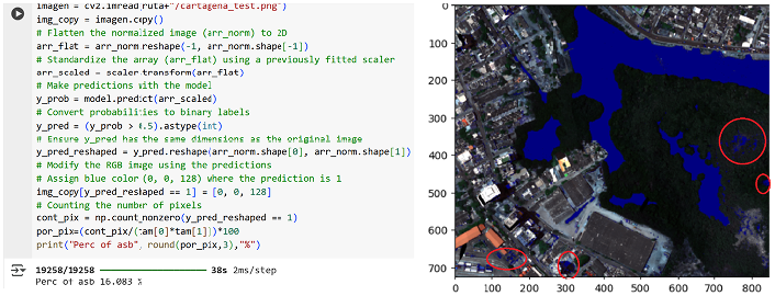
Based on Figure 10, it is possible to observe how the ANN model detected on the reference hyperspectral image a percentage of 16.083% of water body pixels. Despite the above and considering that with respect to the SDS method, the ANN model detected 2.709% more water body pixels, it can be appreciated how the ANN model also makes some additional errors to those presented by the SDS model. Likewise, it is possible to appreciate how both methods show continuous detection of water body pixels.

Likewise, in order to evaluate the computational efficiency of the two methods considered in the present article, multiple repetitions of the methods (25, 50, 75 and 100) were performed on a region of the image of 50x50 pixels and 380 reflectance bands in order to identify the average time per repetition and the total average time employed by each method in processing the selected region of the image. For the implementation of the multiple repetitions of the two methods, the advantages provided by the timeit library were leveraged, which allows performing multiple executions of a method and obtaining the time employed from the multiple executions.

Thus, Figure 11 presents the times obtained by each of the two evaluated methods in the 4 repetitions performed.

Note: Own elaboration

Figure 11 Comparison of average processing times per repetition 

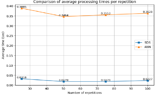
Based on Figure 11, it is possible to appreciate how the SDS method consistently obtains significantly lower processing times than the ANN method for processing the image region. The SDS method times remain below 0.035 seconds in all evaluated repetitions, oscillating between 0.0178 and 0.0318 seconds, while the ANN method presents considerably higher times, varying between 0.3464 and 0.3885 seconds throughout the different repetitions. The analysis of the averages reveals that the SDS method reaches an average time of approximately 0.022 seconds, in contrast with the ANN method that registers an average of 0.358 seconds. This comparison evidences that the ANN method requires approximately 16.1 times more processing time than the SDS method, which demonstrates the greater computational efficiency of the SDS approach for water body detection. The model's performance showed that using 200 signatures increased the statistical robustness of the classification without compromising efficiency, confirming the suitability of this number compared to smaller configurations. Finally, it is worth mentioning that the experimentation was carried out using the features provided by the Google Colab academic environment, which by default is deployed on a cloud-based Linux server with 12.7 GB of RAM and 225 GB of disk space. In this way, considering the environment's specifications, the efficiency evaluation was performed on a portion of the image, being replicable in other environments with higher performance.

5. Discussion

By way of discussion, in this work the implementation and evaluation of two computational methods (SDS and ANN) for the detection of water bodies in hyperspectral images with 380 reflectance bands was proposed as a contribution, which demonstrated having good effectiveness in the detection of this material, in such a way that the SDS method detected on the reference hyperspectral image a percentage of 13.734% of water body pixels, while the ANN model detected a percentage of 16.083% of pixels of this material. Although the ANN model detected a slightly higher percentage of water body pixels, it was also evidenced that it made more errors in detection than the SDS method, however, both methods were accurate in definitively detecting the zones visually identified as water body pixels. In this way, the previous results allow obtaining two alternatives with good effectiveness for water body detection with respect to what was proposed in (^{Chanchí-Golondrino; Ospina-Alarcón & Saba, 2023}), where although effectiveness was obtained in the detection of water bodies in hyperspectral images through the Fourier phase similarity method, it was necessary to perform an exhaustive band range selection process in which the method would not present overlap. Likewise, based on the effectiveness obtained through the two proposed methods, these constitute a competitive alternative to the use of convolutional neural networks (CNN), which have a high computational cost (^{Ghous, Sarfraz, Ahmad, Li & Hong, 2024}; ^{Huang & Tao, 2024}), which is reduced by the less complex structure of ANNs and by the simplicity of the SDS method, thus providing a better balance between efficacy and efficiency with respect to the aforementioned method.

In this same regard, it was possible to determine by performing multiple repetitions of the two methods (25, 50, 75, 100) on a region of the image of 50x50 pixels and 380 bands, that although both methods have similar efficacy in water body detection, the SDS method is 16.1 times faster than the ANN method, which makes it a great alternative to be used in environmental monitoring applications through hyperspectral images, where models such as convolutional neural networks have limited use, since they tend to be costly in terms of computational resources and processing times (^{Huang & Tao, 2024}; ^{Wang et al., 2022}).

On the other hand, by using free libraries and technologies both in image pre-processing and in the implementation, adjustment and evaluation of the two methods proposed in this work, this research becomes a reference to be extrapolated and adapted in the detection of different materials in hyperspectral images in the academic context. Likewise, given the high cost and limitation regarding the customization of material detection methods by proprietary tools, this work becomes an alternative for institutions in developing countries to experiment openly with hyperspectral images. In this same regard, research that has made use of proprietary tools such as ENVI for material detection (^{Hussein & Fakhri Merzah, 2020}; ^{Sekhon et al., 2024}), can more simply improve the proposed methods through hybridization with other techniques using tools like those proposed in this work. Thus, in this research, the spectral library was used for accessing the spectral band data of the image; the TensorFlow library was used for the implementation, adjustment and evaluation of the proposed model; the numpy library was used for the normalization of the reflectance of the original image and for the implementation of the SDS method; the pandas library was used to load the points with the coordinates of the two groups of sample pixels; matplotlib was used for the generation of the different statistical graphs obtained in this research.

6. Conclusions

Considering a challenge of having computational methods in the context of hyperspectral images that provide a balance between detection effectiveness and computational efficiency, in this work the implementation and evaluation of two computational methods (SDS and ANN) for the detection of water bodies in hyperspectral images of 380 reflectance bands was proposed as a contribution. With respect to the SDS model, it was determined that the method did not present overlap when comparing the 200 sample pixels (100 sample pixels of water bodies and 100 pixels of other materials) with respect to the average or characteristic pixel. Likewise, with respect to the ANN model, it was determined that the model with the best fit was the one that had 380 input neurons, 1 output neuron and two hidden layers of 190 and 60 neurons. Considering that both methods present good and comparable effectiveness in water body detection, these methods become an alternative to be considered in environmental monitoring systems where more complex methods such as convolutional neural networks may be limited due to computational cost. Likewise, given the results obtained, these methods can be considered to be extrapolated in the detection of other materials.

When performing the comparison of the effectiveness of the proposed methods, it was determined that while the SDS method obtained a percentage of 13.734% of water body pixels, the sequential ANN model detected a percentage of 16.083%, that is 2.349% of additional water body pixels. Thus, it was obtained that although both methods detect similar zones of water bodies, the ANN method makes a greater number of errors with respect to the SDS method. However, both methods detect the zones with water body pixels in a defined manner and can be considered as comparable, given the slight difference in detection percentages. In this way, these methods can be disseminated in environmental detection applications, taking into account that the thresholds of the SDS method and the architecture of the ANN model must be adapted to the particularities of the material to be detected.

With regard to computational efficiency, the two proposed methods were evaluated on a region of the image of 50x50 pixels and 380 reflectance bands in multiple repetitions (25, 50, 75 and 100), obtaining that on average the time employed by the SDS method in processing the image region was 0.023 seconds, while the ANN model took on average 0.36 seconds to process the same image, which indicates that the SDS method is 16.1 times faster in processing and detecting water bodies in hyperspectral images of 380 bands. In this regard, although both methods are less complex than models based on convolutional neural networks, the SDS method offers competitive advantages to be used in the context of environmental monitoring based on hyperspectral images.

Additionally, this work demonstrated the relevance and effectiveness of free and open source software tools and technologies for image pre-processing, as well as for the adjustment, evaluation and deployment of the proposed methods. In this way, this work and the considered tools can be taken as reference to replicate or extrapolate experimentation regarding material detection in hyperspectral images, especially by universities and research centers in developing countries, considering the high cost of proprietary tools for processing and analyzing these images. Likewise, with respect to proprietary tools, the hybridization and customization capacity of different computational approaches that open source and free software provides is highlighted, allowing the enrichment of existing methods.

7. Limitations and future work

Considering that one of the limitations of hyperspectral images is the computational cost derived from the large number of bands and their redundancy, this work proposed as a contribution a binary classification approach for the proposed methods, which is more efficient in addressing the dimensionality problem. This binary approach offers significant advantages in terms of computational simplicity, reduced processing time, and ease of result interpretation, making it a practical solution for real-time automatic water body detection applications. However, despite both approaches showing good effectiveness in accuracy, both evaluated methods present classification errors that could be mitigated using multiclass classification approaches, considering that unlike other materials, water sample signatures present disparities in their peaks. In this regard, it would be convenient for future work to combine the multiclass approach with dimensionality reduction methods, taking into account the hardware requirements demanded by these images.

Based on the findings of this research, several future lines of work are proposed. First, expanding the dataset with spectral signatures from different regions, types of water bodies (freshwater, brackish, polluted), and atmospheric conditions is recommended to strengthen the models and test their generalization capability. Additionally, implementing data augmentation techniques and cross-validation could improve the stability of the ANN model. Another interesting direction is the integration of dimensionality reduction techniques such as principal component analysis (PCA), wavelet transform, or autoencoders to reduce spectral redundancy and improve efficiency without sacrificing accuracy. From a computational standpoint, deploying both methods in parallel or distributed architectures (e.g., GPU or clusters) is suggested to evaluate their feasibility for real-time monitoring applications. It is also proposed to explore hybrid architectures combining SDS and ANN to take advantage of the strengths of both. Lastly, the proposed methods could be applied to the detection of other materials or environmental phenomena, such as deforestation, pollution, or microplastic presence.