English (pdf)
 Article in xml format
 Article references
 Send this article by e-mail
 Cited by SciELO
  Cited by Google
  Similars in
SciELO
Similars in
SciELO  Similars in Google
 Permalink
1. Initial Considerations
The demand for fish consumption per capita is proliferating worldwide. This increase is particularly significant in low-income countries, were population growth and rapid urbanization drive animal product consumption, including fisheries.
Despite the growth of the fishing market in recent years, there are still obstacles to international production distribution. According to Valdimarsson (2003), fishing faces significant challenges due to the high import taxes charged by some developing countries, which hinder the entry of raw materials and negatively impact the local market. However, according to Subasinghe et al. (2009), the increased demand for fish meat has driven the growth of fish farming, which has proven to be a promising solution to meet global consumption needs. Raising fish in captivity has reduced production costs and increased competitiveness through prices. As a result, in four decades, aquaculture has come to represent 45% of the world's production of fish for consumption.
Production performance, combined with demand and trade in fish, has driven the global fish market, making it one of the most traded food commodities. Fish trade increasingly improves food systems, benefiting local economies and importing countries. In this context, developing countries generally export high-value fish to developed markets, with lobster standing out in this category of high-value products (Tran et al., 2019).
With vast fishing potential along its coastline, Latin America has adopted aquaculture in its territories. Hernández-Rodríguez et al. (2001) report that aquaculture began in the region in the 1940s, initially intending to populate local ecosystems. It was only in the 1960s and 1970s that Latin American countries began to develop aquaculture to produce food for domestic consumption and export, marking a modernization process in the region's fishing economy.
The prospect of modernizing and overcoming challenges in the fishing sector is essential for Brazilian states that depend heavily on this economic activity to develop and increase their export competitiveness. Brazil has two strands of the fishing industry, each with distinct and complementary economic roles. Although aquaculture is one of the fastest-growing economic activities in the country's food sector, marine extractive fishing stands out on the national agenda due to capturing species with high commercial value. It is important to emphasize that even though aquaculture is one of the fastest-growing economic activities in the Brazilian food sector, the most important fish on the national agenda is lobster, a type of crustacean caught by marine extractive fishing that has high commercial value (Farias & Farias, 2018).
However, this segment of Brazilian export trade has faced growth difficulties due to overfishing and the devaluation of the product's price on the international market (Almeida et al., 2021). This makes the locations that depend on this trade vulnerable, depending on both a price recovery and a favorable exchange rate to make exports viable.
In the lobster fishing segment, the state of Ceará stands out. In this state, fish is of great relevance to the trade balance, in addition to being the state that exported the most fish in the country in 2022 among Brazilian states, with 25.19% of the country's total exports. In this state, the fishing market generates around 57 thousand jobs (Ramos et al., 2023).
In this sense, this article seeks to answer the question: Are lobster exports in Ceará affected by price changes and the exchange rate?
To answer this question, we used the vector autoregressive (VAR) model, which has been used recurrently in the literature to study the commodity market in general and the price dynamics of diverse types of fish. Mafimisebi (2012), for example, uses a VAR model to analyze the price dynamics in the dried fish market in Nigeria, revealing that 59.1% of the markets are spatially integrated in the long term.
Fernández-Polanco (2021) uses VAR to analyze the price dynamics of the sea bream (Sparus) market. Murata) in Spain. In short, the authors conclude that prices are transmitted from retailers and wholesalers to farmers in the domestic value chain.
Likewise, García-Del-Hoyo (2023) uses the VAR model to analyze the transmission of price volatility of fresh anchovies in Spain between markets in the value chain. The results achieved allow us to infer that the market with the most terrific price volatility is the one where the product is passed on to large traders (first-hand sales), followed by the wholesale market and, finally, the retail market.
As highlighted in the literature, this model has proven effective in analyzing price volatility in the fish market. It is frequently used in empirical studies demonstrating its ability to capture complex price dynamics and macroeconomic variables. Thus, its approach in this study is justified.
Thus, in addition to this introduction, the second section presents the methodological procedures, the third section presents the results and discussions, and the fourth section presents the final considerations.
2. Methodological procedures
This section will present the methodological procedures adopted in this study. The purpose is to answer the research question and help understand the study object analyzed here.
2.1. Variables and database
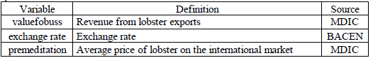
To meet the objective proposed in this study, monthly data were selected from January 2000 to August 2023. Table 1 below shows the variables used in this study, with their respective data sources and expected results.
Table 1: Variables used in the study, definition of variables, and source of available public data.
Source: own elaboration
The vector autoregressive (VAR) econometric model is widely used in the literature on international commodity trade (Felipe, 2013; Castro et al., 2018; Aidar & Deus, 2019; Fernandez, 2020). There is consensus in the literature on the need to begin analytical treatment through stationarity tests. From these tests, it is possible to identify whether the variables have a unit root. These authors conclude that it is only possible to proceed with the VAR if there is stationarity in all variables. Furthermore, after unit root tests, it is necessary to carefully choose the number of lags present in the estimates to develop a good model. However, the Akaike information criteria (AIC), Schwarz's Bayesian criterion (BIC), and the Hannan -Quinn (HQ) become indispensable, and the results of these tests will determine the number of lags that the VAR will have (Akaike, 1974; Schwarz, 1978; Hannan & Quinn, 1979).
From the explanation for using the VAR model, it is possible to state that the model in question meets the demands proposed for the objective proposed in this article since it allows observing the dynamic interactions between the endogenous variables without an immediate need to define causality between them. Prior to its application, the unit root evaluates, and the cointegration test was performed (to define whether the VAR model or the vector error correction model (VEC) will be used); and, after its application, the Granger causality test, the impulse response function, and the variance decomposition were performed. Finally, the forecasts were made using the VAR model.
2.2.Unit root test
The unit root test is a procedure that precedes the choice of the model and its application. It is necessary to determine whether the time series is stationary.
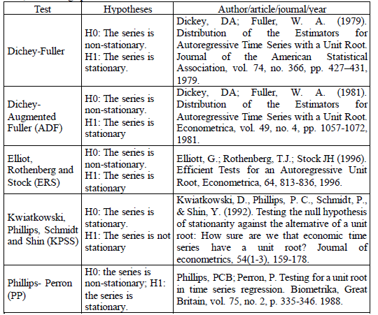
The tests performed to determine whether there is stationarity in the time series were the Dichey-Fuller, Augmented Dichey-Fuller (ADF), Elliot, Rothenberg, and Stock (ERS), Kwiatkowski, Phillips, Schmidt, and Shin (KPSS) and Phillips-Perron (PP) tests, as shown in Table 2 below.
Table 2: Unit root tests applied to time series: Revenue from lobster exports, exchange rate, and average price of lobster from Ceará on the international market
Source: prepared by the authors
All these tests are used to verify whether the observed series is stationary, given models in which the variables are generated by Autoregressive processes of order p, the variables may or may not have a unit root. In this way, it is possible to include the difference in the lagged variable based on the test results, ensuring the preservation of the white noise condition. The unit root tests were performed in the R software with the 'urca' package.
2.2.1. Dickey-Fuller test:
Dickey -Fuller test can be represented mathematically, according to equation 1, below:

Where: yt is the variable under study, Ayt is the first -order difference of the variable (yt -yt-i), t is a time trend (optional), a and ß are coefficients of the constant and the time trend, respectively, y is the coefficient associated with the level of the lagged series (checks if the series has a unit root), St is the random error term.
2.2.2. Dickey-Fuller Test (ADF):
The Dichey-Fuller (ADF) test is expressed by the following mathematical equations:
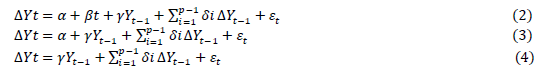
where: yt is the variable under study, Ayt is the first-order difference of the variable (yt -yt-1), t is a time trend (optional), a and ß are coefficients of the constant and the time trend, respectively, y is the coefficient associated with the level of the lagged series (checks if the series has a unit root), 5¡ are the coefficients of the lagged differences of order i, εt is the random error term.
2.2.3. Elliot, Rothenberg, and Stock Test (ERS):
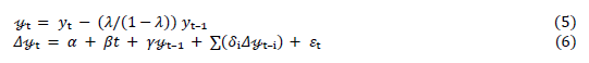
The ERS test can be mathematically defined as in equations 5 and 6 below:
where:
 t is the smoothed time series, λ is the chosen smoothing value (e.g. λ = 7 is a common value), the remaining parameters are defined as in ADF.
2.2.4. Kwiatkowski, Phillips, Schmidt, and Shin Test (KPSS):
The KPSS test has its mathematical definition, according to the demonstration presented in equation 7, below.

where: yt is the variable under study, α is the intercept (constant), ßt is the time trend, rt is a random walk with zero mean, St is the error term.
2.2.5. Perron (PP) test:
The PP test can be mathematically defined as in equation 8 below:

where: yt is the variable under study, Ayt is the first-order difference of the variable (yt -yt-1), t is a time trend (optional), a and ß are coefficients of the constant and the time trend, respectively, y is the coefficient associated with the level of the lagged series (checks if the series has a unit root), St is the random error term.
2.3. Johansen cointegration test - Multivariate model
Based on the results presented by the unit root test, the next step was to apply tests that show whether there is a long-term relationship between the variables in the model. To obtain this result, it is necessary to apply for the cointegration test (Johansen, 1988). The analysis aims to determine the presence or absence of multiple cointegration vectors in a Vector Autoregressive (VAR) model. This model is used in conjunction with error correction mechanisms, known as Vector Error Correction Models (VECM). The mathematical representation of this model can be expressed by the following equations.
Let there be a VAR(p) model, where:

where: yt is a vector of n endogenous variables (nx 1), A¡ are coefficient matrices (nxn) for each lag i, εt is an error vector (nx 1) that is considered white noise.
Error) Model Correction Model) can occur, according to the equation below:

where: Δyt represents the first differences of yt, Π is the long -term matrix (nxn) that contains information about the cointegration between the variables, IT are the short-term matrices (nxn) for each lag Γ i, St is the error vector (nx 1).
Thus, it is possible to perform the decomposition of Matrix n, as follows:

where α (nxr) is the matrix of adjustment coefficients, representing the speed of adjustment to long-term equilibrium, ß (nxr) is the cointegration matrix, where each column of ß represents a cointegration vector, and r is the number of cointegration relations.
Therefore, the Johansen Test can be defined in the two steps below: Trace Test, according to the equation below:

for i = r+1 to n, and Maximum test Eigenvalue Test (Maximum Eigenvalue Test), according to the equation:

where: T is the number of observations, λi are the estimated eigenvalues of the matrix n.
2.4.Granger Causality Test
As proposed in this article, the Granger test (Granger, 1969) will be performed. This test is widely performed in econometric studies on time series. According to the author's approach, correlation alone cannot necessarily imply causality. Granger (1969) explains that the statistical discovery of the relationship between variables is not sufficient to determine a cause-and-effect relationship. Thus, the author suggests that the possibility of the existence of this cause and effect is only valid if past values represented by X t _ 1 collaborate in the prediction of present values Y t . In other words, following Granger's (1969) line of reasoning, a causal relationship between the series is necessary, which cannot be determined solely by a statistical correlation relationship.
Therefore, the mathematical equations responsible for expressing the cause-and-effect conditions can be expressed as follows.

The two equations above represent causality relationships in the Granger sense, μ it , in theory, incorporating uncorrelated noise. In equation (10), it is assumed that the current values of the variable X t are linked to the past values of the variable X t _ 1 , as well as to the lagged values of the variable Y t . In equation (11), represented by Y t , a similar pattern is reflected, where the current values of Y t are related to the lagged values of the variable Y t _ 1 , as well as to the lagged values of the first variable X t . Thus, Granger causality can be identified in the series used in this work as unidirectional and bidirectional.
2.5.Impulse response function
The impulse response function is applied to time series to measure the effect that an endogenous variable has on the other variables in the model. The shock can be applied to any of the variables, the only condition being that it is endogenous to the model. Thus, the result of this shock may affect all endogenous variables and the variable used to apply the shock (Engle & Granger, 1987).
The impulse response function is as follows: The impulse is applied to an endogenous variable in each period t. For example, if the shock is applied to the variable a 1 at time t=0, even if it is applied to only one variable, it can affect all the other variables in the model (Engle & Granger, 1987).
The mathematical representation is as follows, according to equation 12 below:

Where
 represents i, j-th element multiplied by the matrix represented by ψs expanded from an impulse made at time t. It is important to emphasize that for this interpretation to be valid it is necessary that the Var(α
t
) = Σdiagonal matrix where the elements related to a
t
are not correlated.
represents i, j-th element multiplied by the matrix represented by ψs expanded from an impulse made at time t. It is important to emphasize that for this interpretation to be valid it is necessary that the Var(α
t
) = Σdiagonal matrix where the elements related to a
t
are not correlated.
2.6. Variance Decomposition of Forecast Error
Variance decomposition of forecast error is a primary test when using the VAR model (Sims, 1980). According to Aidar and Deus (2019), analysis through variance decomposition seeks to determine the percentage of forecast error variance attributable to each endogenous variable.
For De Souza (2018), the decomposition of the variance of the forecast error and the impulse response function allows us to assess the relevance of the effects of external shocks on each of the variables in the model. It provides the percentage of the variance of the forecast error of each variable in the different future periods that can be attributed to each external shock.
The mathematical representation can be expressed as follows, according to equations 13 and 14, below:
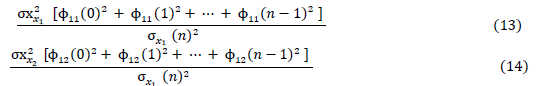
Where, σx𝑥12is the variance of the shocks (or innovations) of the variable 𝑥1. In other words, is the intrinsic variability of the shocks that affect 𝑥1; 𝜙11 (k) are the impulse response coefficients. These coefficients measure the effect of a shock at x 1 at time t on the variable 𝑥1in the subsequent periods t + k; ϕ11(0)2 + ϕ11(1)2+ ⋯ + ϕ11(𝑛−1)2is the sum of the squares of the impulse response coefficients up to period n-1 . The sum of squares is used to measure the cumulative contribution of an initial shock over several periods; σ𝑥1 (𝑛)2is the total variance of the forecast error of 𝑥1over the horizon of n periods. This considers all sources of variability that affect the forecast of 𝑥1over time.
2.7.Vector Autoregressive Model - VAR
After explaining the tests in the subsections above, once the VAR model has been estimated, we now seek to apply the forecasts from the model. This model is widely used in time series because it has the characteristic of capturing interrelated dynamic effects simultaneously (at the same time) of the variables to be analyzed. The estimates are made through Ordinary Least Quadratics - OLS and are represented by three independent and interrelated equations (Sims, 1980).
VAR is represented mathematically as follows:
In matrix form, the VAR takes the following form:

In which 𝑋𝑡represents an autoregressive vector (Nx1) of order 𝜌;𝛼0 is a vector (Nx1) of intercepts;Φ𝑖 is a matrix of order parameters (nxn); and 𝜀𝑡denotes the error term where 𝜀𝑡~𝑁(0,Ω). Based on these settings, the VAR proves to be indispensable for the analysis of the interactions proposed in this work, since it allows us to observe the dynamic relationships between the endogenous variables considered, without the obligation to define the causality between them previously. The following section addresses the results of the analyses and estimates outlined in the methodological procedures presented in this section.
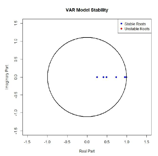
After estimating the VAR Model, its stability test was performed, as shown in Figure below.
Figure 1: VAR model stability test
According to figure 1, all eigenvalues are stable and are within the unitary cycle, showing that there are no problems.
3. Econometric results for lobster exports from Ceará 2002-2023.
Table 1 shows the values of the logarithm of the exchange rate, average price and revenue from lobster exports. According to the results shown in the Table, the minimum values for the exchange rate, average price and export value were 0.4418; 1.204 and 6.377, while the average values were 10.144; 2.274 and 14.657 and the maximum values of the logarithm were 1.7529; 3.828 and 16.494 respectively.
Table 1: Descriptive statistics of the logarithm of the exchange rate, average lobster price and export revenue (U$S)
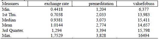
Source: prepared by the author, 2024.
One result that draws attention is the logarithm of the value of exports, as it presents a large discrepancy regarding its maximum and minimum values. This may have caused more significant variability throughout the series treated in this study.
The time series analyzed covers the period from January 2000 to August 2023. This period comprises the equivalent of 272 observations, which can be considered a good number of observations for using econometrics in time series.
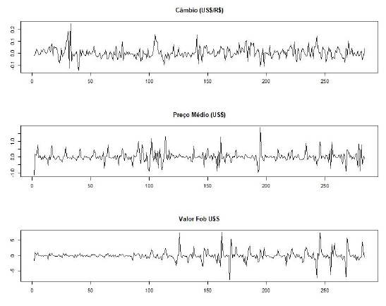
Graph 1: Differentiated series - exchange rate, the average price of lobster exports and export revenues (US$)
As we can see, Graph 1 shows that the logarithm of the exchange rate has a movement like the logarithm of the average price of lobster. By preliminary analysis of the series, it is possible to see that as the logarithm of the exchange rate increases, the average price falls. Likewise, the average price increases when the exchange rate decreases, suggesting a possible inverse relationship between the two variables. When analyzing the third graph referring to the average revenue from exports, we notice a relationship of minor sensitivity up to the observation number 100, and from there, more significant oscillations are observed, suggesting a more contemporary relationship with the other variables.
According to Panisson (2018), to estimate the VAR model, it is necessary to perform the unit root test to confirm whether the series in question is stationary or not. The most widely used test to find out whether the series has stationarity is the Dickey-Fuller (ADF) test. However, to ensure greater security in the results, the Dickey-Fuller augmented GLS (DF-GSL) test, Elliott-Rothenberg-Stock test - with constant, Kwiatkowski -Phillips-Schmidt-Shin test - KPSS - with constant and the Phillips- Perron (PP) Unit Root Test were also performed.
Table 2 below shows the results found for the variables' logarithms from the tests mentioned in the previous paragraph for a confidence interval of 1%, 5%, and 10%.
Table 2: Unit Root Tests applied to the series in differences: exchange rate, average
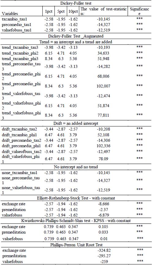
Source: prepared by the author, 2024.
It is important to highlight that the null hypothesis of the ADF, PP, DF-GLS, and ERS tests is the presence of a unit root in the series, which indicates that the series is not stationary. In contrast, the KPSS test assumes as a null hypothesis that the series does not have a unit root, which means that the series is stationary.
As can be seen, after the tests, the Dickey-Fuller test proved not to have a unit root in the series since the values found for the variables exchange rate, average price, and value of exports were lower than the critical values at 1%, 5%, and 10%. The Augmented Dickey-Fuller test is nothing more than an extension of the previous test but more robust. After the analysis, the stationarity of the residuals obtained by the Ordinary Least Squares method was verified. The Tau statistic was used to test the slope, resulting in the rejection of the null hypothesis, which indicates that the series does not have a unit root and, therefore, is stationary.
The Elliott-Rothenberg-Stock tests also showed no unit root for the model. In this test, attention is drawn to the values found for the exchange rate and the value of exports, which were well away from zero, while the average price obtained a value closer to zero. The Kwiatkowski -Phillips-Schmidt-Shin KPSS test had positive values between 0 and 1, confirming what was presented in the previous test. That is, there is no unit root in the time series. Finally, the Phillips-Perron (PP) Unit Root Test showed negative parameters smaller than zero, leading to rejecting the null hypothesis, as occurred in the ADF, DF-GLS, and ERS tests.
After performing the stationarity tests, it is necessary to determine the order in which the VAR model lags are chosen. The AIC (Akaike) and BIC (Bayesian) criteria were used. Information Criterion) and HQ (Hannan -Quinn): These criteria define the appropriate number of lags in the VAR model.
Table 3: Tests for determining the order and choosing the VAR model - AIC, BIC, HQ, and M(p).
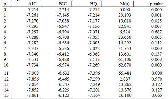
Source: prepared by the authors, 2024.
Based on the values presented in Table 3, a VAR (11) model with 11 lags was selected since the lowest values of the Akaike and Hannan -Quinn information criteria indicated this specification.
3.1. Cointegration test result: trace and maximum eigenvalue tests
No unit root was found in the logarithm of the model's tested series, as shown in Table 2. Therefore, the next step is the co-integration test. According to Sibin, Da Silva Filho, and Ballini (2016), the stage begins with evaluating the proposed model through the first difference analysis. This stage consists of examining the model's stability.
The Johansen co-integration test was performed to assess the existence of a long-term relationship between the variables. Initially, the hypothesis r<=2 was considered, analyzing the possibility of up to two cointegration vectors. Then, the hypothesis r<=1 was tested, considering the existence of a single cointegration vector. Finally, the null hypothesis verified the presence of cointegration between the model variables, with significance levels of 10%, 5%, and 1%.
Table 4: Result of the Johansen cointegration test: trace and maximum eigenvalue tests.
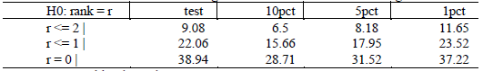
Source: prepared by the author, 2024.
As can be seen in Table 4, the Johansen cointegration test showed that the series are cointegrated with each other. Thus, we can conclude that, given the number of cointegration vectors in the Table above, it is possible to see integration between the model variables at 1%, 5%, and 10% significance. In other words, there is a possible long-term relationship between them, so we used the VAR model to adjust the time series proposed by this study.
3.2. VAR model stability test
In the context of the VAR model, it is vital to ensure the absence of residual correlation. When examining the correlogram of the residuals of the VAR model, as shown in Figure 2, one observes the absence of residual correlation in the series. What is observed are isolated occurrences. Therefore, rejecting the null hypothesis of the absence of correlation in some specific lags is impossible. However, considering the lack of pattern among the monthly periodicities of the series analyzed, it is interpreted that such correlations are only due to the natural characteristics of time series of this nature.
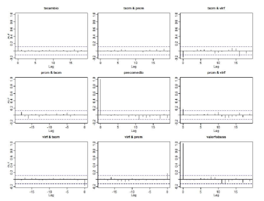
Two more tests were applied to complement the correlogram to ensure no autocorrelation in the model. The first test is the Portmanteau test, which has the non-existence of non-contemporaneous autocorrelation as its null hypothesis. The LM test tests the null hypothesis of the non-existence of serial correlation in the residuals of the first-order model. Both tests confirmed the non-existence of residual autocorrelation.
3.3. Granger Causality Test
Granger (1969) developed a test known as the Granger causality test, which is based on the premise that the future cannot influence the present or the past (Felipe, 2013). To better understand whether a occurs after ß, it is understood that a cannot cause ß. In the same way that if a happens before ß, this does not necessarily imply that a is the cause or influences ß. It is necessary that regardless of whether a happens before ß or after ß or both happen simultaneously, a does not influence ß nor does ß influence a.
As shown in Table 5 below, the Granger causality test was applied to the three variables to verify their interdependence. The first analysis, which refers to the exchange rate explained by two lags of the exchange rate plus two lags of the average price, results in a P value associated with more than 5%, thus failing to reject the null hypothesis, indicating that we cannot state that the exchange rate Granger causes the average price. In other words, a shock in the lagged values of the exchange rate variable does not impact the average price of lobster exports from Ceará. When an exchange rate shock is made concerning the value of exports, we also have a P value associated with more than 5%. Therefore, in this case, the null hypothesis is not rejected. That is, there is no causal relationship, in the Granger sense, that the exchange rate causes revenue from lobster exports to the international market.
Table 5: Granger causality test for the exchange rate, the average price of lobster
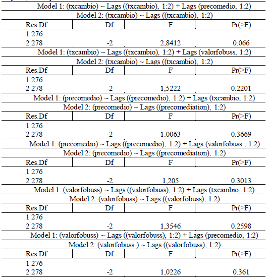
P=., sig 0.1; p=*, sig=0.05; p=**, sig=0.01, p=***, sig=0.001
Source: prepared by autoes, 2024.
When applying a shock using two lags of the average price variable together with two lags of the exchange rate and, subsequently, with the value of exports, the result showed that the p-value associated with the average price, both with the exchange rate and the value of exports, was higher than the 5% significance level. This indicates that the null hypothesis cannot be rejected. Thus, it can be concluded that the average price does not Granger cause either the exchange rate or the value of exports, showing that a shock in the lagged values of the average price variable does not impact the exchange rate or the value of exports.
Finally, the impact of the export value variable on the number of lags with the exchange rate and average price variables was analyzed. As a result, a p-value associated with significance more significant than 5% was found for both variables. Furthermore, the null hypothesis was not rejected, concluding that export revenue does not Granger cause the exchange rate, as it does not Granger cause the average price. In other words, the export value series has no temporal precedence regarding the exchange rate or the average price.
The results suggest that lobster exports from Ceará during the analyzed period are more closely related to the supply and demand components than to the macroeconomic variables tested. In other words, exports are random and more closely related to the fishermen's supply capacity and the market's demand capacity.
3.4. Impulse response function
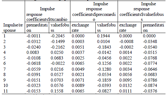
Next, the responses of each variable in the model to unexpected shocks on themselves and the other variables were analyzed. Table 1A, in the appendix, shows numerically the behavior of the three variables to the impulse response data on themselves and on the other endogenous variables in the model over eleven periods. The same results can also be visualized graphically in Figure 3.
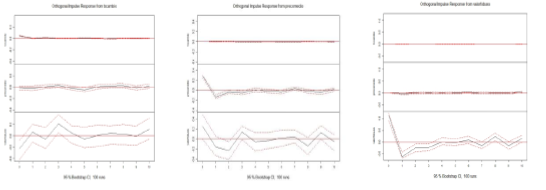
Figure 3: Impulse Response Function for the variables, exchange rate, average price, and export revenue.
As illustrated in Figure 3, a shock to the exchange rate generates an initial positive response from the variable itself in the first few months, but this effect quickly dissipates. This same shock, however, does not impact on the average price of lobster on the international market, whose series remains stable. Similarly, export revenue reacts negatively initially, but this influence diminishes rapidly over time. The results for the exchange rate shock indicate that, initially, it exerts a minimal impact on the variable itself and revenue from lobster exports. However, its influence on the variables is shortlived.
A shock to the average price of lobster on the international market initially generates a positive response only in the variable itself; however, this positive response soon attenuates over time. On the other hand, the exchange rate and export revenue do not significantly react to this shock. In short, an increase in the average price of lobster has a positive impact only on the price itself, and, as a shock to the exchange rate, this influence is short-lived.
Finally, a shock to lobster export revenue presents a response only in the variable itself, with an initial positive effect in the first few months. However, this effect dissipates over time as with the other shocks analyzed. The other variables do not present a significant response to the shock to lobster export revenue. In short, a shock to lobster export revenue exclusively affects the variable itself.
Therefore, it is concluded that the dynamics of lobster exports show a limited response to shocks in international prices and the exchange rate, with responses being restricted to the variable itself. The effects of these shocks are transitory and quickly dissipate over time, indicating that volatility in lobster exports is not significantly transmitted to the other economic variables analyzed. Thus, as in the Granger causality test, it leads to the inference that the Brazilian lobster trade is more closely linked to supply and demand than to the economic variables analyzed here.
After performing the impulse response function, the next step is to perform the variance decomposition. Sibin, Da Silva Filho, and Ballini (2016) report that variance decomposition makes it feasible to determine the proportion of the variance of forecast errors that can be associated with unanticipated shocks of the variable in question and of the other endogenous variables of the system on an individual basis.
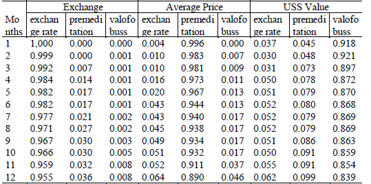
3.5. Forecast Error Variance Decomposition
Table 1B, in the appendix, presents the results of the variance decomposition of the forecast error for twelve periods for the variables exchange rate, average price, and export revenue. In the exchange rate component, as expected, its decomposition explains 100% of its forecast error. At the end of the period analyzed, this value remains high, falling only to a percentage of 95.5%. The average price explains 0% in the first period and has little influence over time, explaining only 3.5% of the exchange rate forecast error. On the other hand, the value of exports has an even more negligible impact, causing less than 1% of the variance of the exchange rate forecast error.
The variance analysis applied to the average price component revealed very low percentages over the 12 periods studied for the other variables. At the beginning of the series, the exchange rate variable contributed only 0.4% of the average price forecast error, increasing to 6.4% after 12 periods. The average price variable is responsible for most of the forecast variance, accounting for 99.6% in the first period, and this percentage decreases to 89% as the forecast horizon extends. In contrast, the value of exports initially does not influence the average price forecast error, but this contribution increases to 4.6% over the cycles.
The export value variable is the one that presents the most significant contribution of the other variables in its variance forecast error at the end of the twelve periods compared to the other variables. Initially, the export value explained 91.8% of its forecasts, while the exchange rate and the average price contributed to 3.7% and 4.5%, respectively. After the 12 periods, the ability of the export value to explain its variance decreased by 7.9%, falling to 83.9%. As expected, the other variables showed an increase: the exchange rate rose to 6.2%, and the average price, which had the most significant increase, began to explain 9.9% of the variance error of the export value.
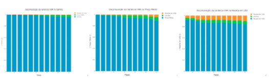
Figure 4 above shows how the variance decomposition of the forecast error is distributed. As can be seen, of the three variables, the exchange rate is almost unaffected by the other variables. The shock presented by the average price and the value of exports, added together, explains only 5% of the forecast error of the variable analyzed. The shock in the average price component shows a more significant impact than the previous variables since it added to the exchange rate and the value of exports, which explains 11% of the average price.
Of all the endogenous components presented, the value of exports was the one most influenced by the other variables when analyzing the forecast error. At the end of the period, this lost more than 15% of its explanatory capacity; this loss can be seen in Graph 3 of Figure 4.
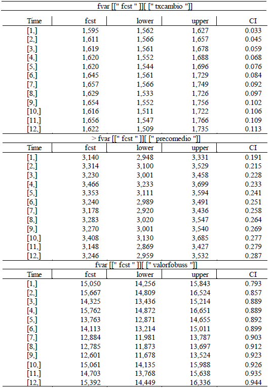
3.6. VAR Predictions
After all the tests have been performed, we can proceed with the forecasts using the VAR model. Table 1C in the appendix presents the estimates of each variable over 12 months. As can be seen, the exchange rate has a forecast within the confidence interval, both in the upper and lower bands, with a confidence level of 95%.
The VAR model also presents satisfactory results for the other two variables in the series, with predictions within the 95% confidence interval in both the upper and lower bands. This demonstrates the model's robustness for the variables analyzed.
Figure 5 shows how the forecasts are distributed in the VAR model, referring to Table 1C of the appendix. As can be seen in the first two graphs, which correspond to the exchange rate and the average price, respectively, the blue dotted line behaves within the red lines.
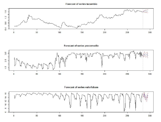
Figure 5: Forecasts for the impacts of the exchange rate on the price and the total value of revenues from lobster exports from Ceará using the VAR model.
The blue line in the third graph in Figure 5 remains within the parameters, although it presents more significant oscillations than the previous graphs. This indicates that, despite the variations, the forecasts remain within a 95% confidence interval, demonstrating the reliability of the estimate obtained from the VAR model.
4. FINAL CONSIDERATIONS
This article aimed to show the relationships between the variables exchange rate and the average price and revenue from lobster exports in the State of Ceará. The study's motivation was that Ceará is the largest lobster producer in Brazil. Thus, this ranking justifies a study of this nature, given the importance of Ceará's exports in this sector for both the country and the state. Furthermore, this analysis contributed to understanding this sector in the fish export trade since it is little explored in the literature and never addressed by the approach presented here.
The responses were obtained through the VAR model. However, before applying the data to the VAR model's econometric modeling, tests were carried out to identify the existence of interrelationships between the three components of the time series and to assess the model's viability for carrying out the analyses.
The unit root test was applied, as suggested in the literature: Dickey-Fuller and Augmented Dickey-Fuller, Elliott-Rothenberg-Stock, Kwiatkowski -Phillips-Schmidt-Shin, and Phillip-Perron. Furthermore, the Johansen trace test was performed to identify the variables' cointegration relationship and choose between the VAR and the VEC. After choosing the VAR, the Granger causality test, the impulse response function, and the forecast error variance decomposition were applied.
The AIC, BIC, and HQ criteria were used to determine the order of the model selection. The AIC and HQ criteria indicated the same order; therefore, they were chosen. From this, a VAR model with eleven lags was estimated.
It was not possible to identify Granger causality between the variables. The test indicated no long-term dependence relationship between the three variables observed in the model. Furthermore, based on the impulse response function, it is concluded that the dynamics of lobster exports present a limited response to shocks in international prices and the exchange rate, with responses being restricted to the variable itself. However, these shocks are transitory and quickly dissipate over time, indicating that volatility in lobster exports is not significantly transmitted to the other economic variables analyzed.
Thus, despite the economic potential of the lobster export sector to Ceará, it faces significant challenges, such as overfishing, which affects the sustainability of catches and, consequently, future exports of the goods. The results of this study suggest that the dynamics of lobster exports from the State of Ceará seem to be more linked to issues related to supply and demand rather than to the behavior of macroeconomic variables that traditionally determine international trade. This conclusion points to the need for strategies that promote sustainable fisheries management, ensuring the continuity of the export sector and reducing vulnerability to fluctuations in supply, which are essential to maintaining Ceará's competitiveness in the international lobster market. In addition, promoting awareness about lobster marketing in the context of favorable exchange rates and international prices is essential.