


 English (pdf)
 Article in xml format
 Article references
 Send this article by e-mail
 Cited by SciELO
  Cited by Google
  Similars in
SciELO
Similars in
SciELO  Similars in Google
 Permalink
1. Introduction
Population aging has traditionally been viewed as a disadvantage for economic growth within mainstream economic thought (Haiming & Zhang, 2015). According to the World Economic Outlook (IMF, 2025) and the report Enhancing Productivity and Growth in an Ageing Society (OECD, 2024), the so-called "silver economy" is emerging as a new axis of structural reorganization of labor markets and aggregate demand, requiring adaptations in public policies and production systems. In this context, understanding the effects of aging on Brazilian economic growth becomes essential, especially amid rapid demographic transition and growing fiscal and social-security challenges (United Nations, 2024).
Several authors argue that population aging may generate labor shortages, contributing to slower productivity growth and exerting downward pressure on aggregate savings. However, the dominant theoretical perspective often overlooks the labor market participation of older adults, as well as their accumulated savings and assets-factors that may shape both the direction and magnitude of aging's economic effects (Haiming & Zhang, 2015). A more comprehensive understanding therefore requires considering not only demographic structure, but also institutional, behavioral, and labor market adjustments.
The international literature on aging and economic growth is broad and heterogeneous. Seminal works such as Bloom, Canning, and Fink (2010)), Lee and Mason (2011), and Acemoglu and Restrepo (2017) generally find neutral or negative effects of aging on per-capita output, mainly through reductions in labor supply and marginal productivity. However, more recent studies-Maestas, Mullen, and Powell (2023); Acemoglu and Restrepo (2022)- introduce important nuances: aging can induce efficiency gains through automation, re-skilling, and capital reallocation, mitigating adverse effects. Reports by multilateral institutions (IMF, 2025; OECD, 2024) reinforce this view, emphasizing that demographic impacts depend largely on active-aging policies and the technological adaptability of economies.
Another aspect to be considered is the demographic transition. According to Vasconcelos et al. (2008), this process has been a central element in understanding population dynamics since the Industrial Revolution. As advances in medicine, sanitation, and nutrition reduced mortality rates and increased life expectancy, infant mortality declined and longevity expanded. However, because birth rates remained high during the early stages of this transition, population growth accelerated rapidly-a phenomenon widely referred to as the demographic explosion. It is precisely this gradual reconfiguration of the age structure, from a predominantly young population to one increasingly composed of adults and older individuals, that gave rise to the contemporary process of population aging.
In Brazil, population aging represents an ongoing structural transformation with direct implications for productivity, savings, and long-term economic growth. Traditional literature suggests that aging reduces labor supply and slows productivity growth, while increasing pressure on social protection systems (Bloom, Canning, & Fink, 2010; Lee & Mason, 2011). However, recent evidence indicates that these effects may vary depending on institutional adaptability, investments in human capital, and the labor force participation of older individuals (Acemoglu & Restrepo, 2017; Maestas, Mullen, & Powell, 2023). This issue is particularly relevant because the country is nearing the end of its demographic dividend, a period marked by a favorable age structure that has supported economic expansion. As the age distribution shifts, Brazil faces a transition that may reshape its long-term growth trajectory (IBGE, 2021).
In response to these demographic changes, recent constitutional reforms-such as the pension reform and the labor market reform-aimed to adjust the social security system to increasing longevity and to introduce greater flexibility in employment relations. These reforms recognize that the economic effects of aging depend on the capacity to retain, retrain, and integrate older workers, thereby mitigating productivity losses or potentially generating gains. This leads to the following research question: Does population aging in Brazil imply increased long-term productivity?
Given that economic growth is constrained by the availability and combination of production factors (working-age population, capital accumulation, and education), the research hypothesis is that population aging positively contributes to Brazil's long-term economic growth, particularly when accompanied by improvements in human capital and labor market adaptation. To test this hypothesis, the study employs an extended Solow Model including the dependency ratio, estimated through Johansen cointegration tests and VECM.
Thus, this study contributes to the literature by providing empirical evidence on the long-term relationship between aging and productivity and offering insights for policymakers. Beyond this introduction, Section 2 outlines the methodology, Section 3 presents and discusses the results, and Section 4 concludes.
2. Methodology
2.1 Theoretical Model
The Solow Model, also known as the Exogenous Growth Model, developed by Robert Solow in 1956, is a widely used model to analyze long-term economic growth. It is based on the idea that economic growth is driven by three main factors: capital, labor, and technology. For Solow (1956), economic growth is a process of change in the composition of the economy, with capital replacing labor. Therefore, population aging mainly affects the labor factor.
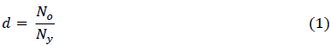
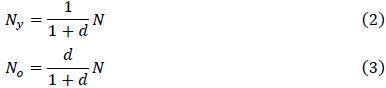
In this work, we followed the procedures indicated by Haiming and Zhang (2015) who introduced the dependency ratio of the Chinese population into the Solow model. Initially, the authors divide the total population (quantity is expressed as N) into young (Ny) and elderly (No). The population aging index adopted by the authors is a dependency ratio (d) represented by the following equation:
Where we can perform the following rearrangements represented by the following equations:
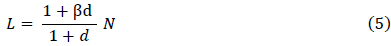
The authors then assume that the labor supply of older people is an exogenous proportion β (0 < β < 1), that all young people participate in the job offer and the population increase is a constant n. With this, they get a μ =
 1which refers to the increase in the dependency ratio, which they take as exogenous to simplify the analysis. The total labor supply of the economy is represented by Equation 4.

After making the rearrangements, the total labor supply in the economy is represented by the equation below:
Assuming that the population growth rate n is constant, the growth rate of the total labor supply is represented by the following equation:
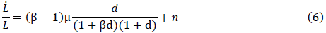
In the basic Solow model, the μ = 0, because it does not take into account the aging of the population. When considering aging, the ц can be positive or negative. Therefore, aging can increase or reduce the supply of labor.
The authors assume a Cobb-Douglas production function with constant returns to scale, where Y represents the gross product of the economy, K represents the total capital stock, A represents technological progress and a represents the relative importance of capital and labor.

Without considering technical progress and depreciation of capital, the capital accumulation equation is represented by K̇̇ = I, where I is the total investment of the economy. As total investment comes from the accumulation of savings (s), including both the savings of young people and the savings of the elderly, the macroeconomic equilibrium condition can be represented by the following equation:

Defining the capital-labor relationship as
 and the income-work relationship

 the following equation is obtained:

It can be seen that there is a unique steady state, represented by the equation below:

The authors were concerned about the effects of population aging on economic growth. Thus, they defined capital per capita as
 and per capita income as

 .Thus, they defined the values for the steady state as presented by Equations 11 and 12.
Where к* represents capital per capita in the steady state and y* represents the steady-state per capita income. This indicates that steady-state per capita income depends on the labor supply rate of older people. (β), savings rate (s), of the dependency ratio (d) and its growth rate (μ), as well as the population growth rate (n). In this way, we can derive the savings rate (s) and the dependency ratio (d), presenting the following equations:
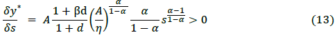
From equation 13, it can be seen that the long-run effect of the savings rate on per capita income in the steady state is positive.

In equation 14, the first term is negative. The sign of the second term depends on the aging rate μ. According to the authors, if μ < 0, then
 This indicates that when population aging is slow, the marginal contribution of the steady-state dependency ratio is negative. If μ > 0, the sign of
 is uncertain. If the aging rate is too fast, then
 This shows that the marginal contribution of the old-age dependency ratio to steady-state per capita income is positive.
For the authors, this result depends on the hypothesis that the elderly also participate in the labor supply and that they have savings, which is proven through empirical analyses. According to this model, the following can be speculated: per capita income, savings rate, and old-age dependency ratio have an equilibrium relationship in the long run. Per capita income is positively correlated with savings rate, and its relationship with the dependency ratio is uncertain.
2.2 Data and Source
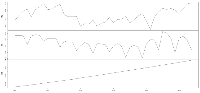
The data are quarterly and cover the period from January 2012 to December 2022, considering the following variables: Iny - represents the logarithm of real GDP per capita, obtained through the ratio of real GDP/total population, with the GDP series being deflated by the Broad Consumer Price Index, as a conversion index to obtain real GDP, Ins - represents the quarterly savings rate in logarithm, and Ind - represents the quotient of the dependency ratio between the inactive population and the active population in logarithm. The observations are obtained from the Continuous National Household Sample Survey, which was implemented throughout Brazil in January 2012, and from the Brazilian Institute of Geography and Statistics.
Given the unavailability of quarterly data for the age pyramid, the quarterly basis of the population distributed by age group is adopted as selective, defined as follows: (i) for the inactive population, considered the group of people aged 60 or over and (ii) for the active population, considered the group of people aged between 14 and 59 years. Table 1 presents the definitions of the variables analyzed in the model, the data sources, and the transformations applied. Table 1 presents the descriptive statistics of the series considered.
Table 1 Descriptive Statistics
| Iny | Ins | Ind | |
| Mean | 9.321 | -1.904 | -1.630 |
| Median | 9.315 | -1.901 | -1.634 |
| Standard Deviation | 0.046 | 0.202 | 0.099 |
| Minimum | 9.226 | -2.386 | -1.786 |
| Maximum | 9.402 | -1.542 | -1.457 |
Source: Prepared by author
Figure 1 illustrates the trajectory of the series in logarithms. It can be seen in the graph that the series Iny e Ins present non-stationarity characteristics. The series Ind presents a trend characteristic due to population growth.
2.3 Empirical Model
Our empirical model is based on the theoretical work developed by Haiming and Zhang (2015) to test the long-term relationship between per capita income, savings rate, and elderly dependency ratio. We can set up an econometric model for these three variables as shown in the equation:

Where Iny represents the logarithm of real GDP per capita, Ins represents the quarterly savings rate in logarithm, and Ind represents the logarithm of the dependency ratio between the inactive population and the active population. The empirical model aims to test the cointegration between variables when two series share a long-term relationship. For this purpose, the Vector Error Correction Model (VECM) developed by Engle and Granger (1987) is applied. In the work, the authors proposed the VECM as a way to estimate a long-term relationship between cointegrated variables. The general form of the Vector Error Correction Model (VECM) is:

Where Δ is the first difference operator, ec t-1 is the error correction term lagged one period, λ is the short-term coefficient of the error correction term (-1 < λ < 0), and u t is the white noise term (error term). Based on the theoretical model proposed by Haiming and Zhang (2015), we will use the VECM model arranged in the following equation:

Where Δ represents the first difference of variables, Лес represents the error correction term, and μ represents the error term of the model.
When applied to population aging and economic growth, VECM allows us to assess how changes in the demographic structure affect the long-term equilibrium of the economy. It considers not only short-term relationships, but also the speed at which the economy returns to its long-term equilibrium state after shocks. In this way, it is possible to identify how changes in the demographic structure affect variables such as consumption, investment, and productivity.
3. Results
The first step of the analysis is to verify the stationarity of the series by means of unit root tests. Next, the criteria for selecting variable lags are verified, and it is verified whether the series considered are cointegrated by means of Johansen cointegration tests. Finally, the error correction model is estimated to find the short- and long-term relationships between the series.
4.1 Unit Root Tests
The concept of stationarity is the main idea that must be taken into account when estimating a time series (Bueno, 2018). For a series to be stationary, there must be no variations in its mean and variance over time, and the covariance must depend only on the distance between two periods. In this sense, to establish the order of integration of the series, the unit root tests ADF, DF-GLS, PP, and KPSS were used. The results, presented in Table 2, show that all the series considered have a unit root at the level when we observe the results of the ADF and DF-GLS tests.
Table 2 Unit Root Tests
| Serie | ADF (1) | DF-GLS (2) | KPSS (3) | PP (4) |
|---|---|---|---|---|
| Iny | 0.3089 | -1.3397 | 0.2203 | -2.1387 |
| Δlny | -6.6453*** | -4.0739*** | 0.1162*** | -7.561*** |
| Ins | 0.2019 | -1.5775 | 0.3897* | -4.6508* |
| Δlns | -14.2761** | -1.7243* | 0.048*** | -10.0376*** |
| Ind | -1.4278 | -0.6298 | 1.2018*** | -9.5458*** |
| Δlnd | 2.6631*** | 0.5305 | 1.4325 | -4.2242*** |
Notes:
(1) Applied to test equations without intercept or trend. Use the Akaike Method - AIC.
(2) Applied to test equations without an intercept. Use the Akaike Method - AIC.
(3) The KPSS test has the null hypothesis of stationarity of the series. Applied to test equations with intercept and trend.
(4) Applied to test equations with intercept and trend. The PP test is most applied to large samples.
Consider rejecting the null hypothesis at significance levels; *, 10%, 5%, and 1% respectively. Note that if you reject H0 at 1% (***) then you reject H0 at 5% and 10%, it will no longer be necessary to add more stars than the three.
Source: Prepared by author
With the test results contained in Table 2, it is possible to see that the series considered are stationary in first difference, I(1).
4.2 Estimation Results
For cases of smaller sample sizes, the literature recommends using a smaller number of lags to help avoid overfitting and improve the generalization of a more parsimonious model. A parsimonious model explains the data with a minimum number of parameters or predictor variables. The idea behind parsimonious models derives from Occam's Law or the law of brevity. According to William of Occam (1320-1349), this law states that, between two explanations for a phenomenon, the simpler one is more likely to be true.
Table 3 presents the results of the lag selection criteria. The Akaike (AIC), Hannan-Quinn (HQ), and Schwarz (BIC) information criteria are used to identify the order p of the VECM model. The AIC, SC, and HQ information criteria indicated the choice of the order p = 4, indicating the lowest calculated value.
Table 3 Choice of Lag Orders
| Lag (p) | AIC | HQ | BIC |
|---|---|---|---|
| 1 | -32.685303 | -32.318915 | -31.671975 |
| 2 | -32.796516 | -32.292733 | -31.403190 |
| 3 | -33.411996 | -32.770819 | -31.638673 |
| 4 | -33.943000 | -33.164427 | -31.789678 |
Source: Prepared by author
After selecting the lag order for the variables, we estimate the possible cointegration relationships, using the work of Johansen (1988) as a reference. The Johansen Cointegration Test is a statistical test that allows us to verify whether there is a long-term equilibrium relationship between two or more economic variables.
According to Ferreira et al. (2017), the results provide two statistics that allow a sequential procedure to be carried out to infer the number of cointegration vectors (r). The first, regarding the number of cointegration vectors, is called the trace (or rank) statistic. The second, the comparison between two values of r e r + 1, is called the maximum eigenvalue statistic. The test has as its null hypothesis r = 0, where r represents the non-existence of cointegration relations. When r <= i, it is equivalent to i or fewer cointegration relations.
In Table 4, we estimate the existence of two cointegration vectors according to the maximum eigenvalue statistic at the 5% significance level. Since we have only three variables, there will be at most two cointegration relations.
Table 4 Johansen Cointegration Test
| Number of r | t-test | Trace Statistic (Rank Statistic) Critical Value (5%) | Probability | t-test | Maximum Eigenvalue Statistic (Eigenvalue - Lambda Max) Critical Value(5%) | Probability |
|---|---|---|---|---|---|---|
| r = 0* | 43.8719 | 29.7970 | 0.0007 | 28.4406 | 21.1316 | 0.0039 |
| r <= 1 | 15.4313(1) | 15.4947 | 0.0511 | 15.4305 | 14.2646 | 0.0326 |
| r <= 2 | 0.000806 | 3.8415 | 0.9785 | 0.000806(2) | 3.8414 | 0.9785 |
Note 1: *Denotes that there is rejection of the hypothesis at the 5% level. The criterion with intercept and without trend was adopted.
Note 2: The criterion with intercept and without trend was specified.
*1) Trace Statistics indicates a cointegration vector at the 5% level.
*2) Maximum Eigenvalue Statistics indicates two cointegration vectors at the 5% level.
Source: Prepared by author
Once the cointegration vectors have been defined, we proceed to estimate the error correction model to find the long-term relationship between the variables lny, lns, and lnd. According to the estimated error correction term (18), we have a long-term equilibrium relationship that can be obtained according to the cointegration equation (19).

The initial results of the cointegration relationship suggest that, in the long run, the increase in per capita income is negatively correlated with the savings rate and positively correlated with population aging. If other conditions remain unchanged, when the savings rate increases by 1%, per capita income will decrease by about 0.18%. With other conditions unchanged, if the old-age dependency ratio increases by 1%, per capita income will increase by about 2.05%. Table 5 presents the results of the VECM model estimations.
Table 5 Estimation of the VECM Model Equations
| Variables | Cointegration Equation | ||
|---|---|---|---|
| lny(-1) | 1.00000 | ||
| lns(-1) | 0.18126 | ||
| (0.08047) | |||
| [2.25252] | |||
| Ind(-l) | -2.051634 | ||
| (0.32693) | |||
| [-6.27539] | |||
| С | -12.29315 | ||
| Error Correction | d(Zny) | d(Zns) | d(Znd) |
| CointEq1 | -0.269744 | -1.539552 | 0.000425 |
| (0.13888) | (0.44926) | (0.00028) | |
| [-1.94231] | [-3.42686] | [ 1.53311] | |
| D(Zny(-1)) | 0.007069 | 0.836739 | -0.00152 |
| (0.209170) | (0.676640) | (0.000420) | |
| [ 0.03379] | [ 1.23662] | [-3.63892] | |
| D(Zny(-2)) | 0.154439 | 1.002256 | -0.001227 |
| (0.177460) | (0.574070) | (0.000350) | |
| [ 0.87028] | [ 1.74588] | [-3.46161] | |
| D(Zny(-3)) | -0.378322 | -0.670683 | -0.000948 |
| (0.187980) | (0.608100) | (0.000380) | |
| [-2.01257] | [-1.10291] | [-2.52397] | |
| D(Zny(-4)) | 0.016415 | -1.397815 | -0.001719 |
| (0.18371) | (0.59430) | (0.00037) | |
| [ 0.08935] | [-2.35204] | [-4.68540] | |
| D(ZnS(-1)) | 0.063821 | -0.276812 | -0.000120 |
| (0.04906) | (0.15870) | (0.000098) | |
| [ 1.30095] | [-1.74428] | [-1.22995] | |
| D(ZnS(-2)) | 0.082831 | -0.206065 | 0.000389 |
| (0.04288) | (0.13870) | (0.000086) | |
| [ 1.93181] | [-1.48563] | [ 4.54229] | |
| D(ZnS(-3)) | 0.05105 | -0.099864 | 0.000133 |
| (0.05692) | (0.18415) | (0.00011) | |
| [ 0.89681] | [-0.54231] | [ 1.17371] | |
| D(ZnS(-4)) | 0.049657 | 0.533945 | 0.000357 |
| (0.04614) | (0.14925) | (0.000092) | |
| [ 1.07629] | [ 3.57748] | [ 3.87245] | |
| D(Znd(-1)) | -42.793510 | -356.4069 | 0.374048 |
| (69.2170) | (223.912) | (0.13823) | |
| [-0.61825] | [-1.59172] | [ 2.70597] | |
| D(Znd(-2)) | -45.00243 | 152.37800 | -0.37476 |
| (85.48) | (276529.00) | (0.17) | |
| [-0.52646] | [ 0.55104] | [-2.19525] | |
| D(Znd(-3)) | 73.81245 | -68.48359 | 0.52608 |
| (79.4575) | (257.040) | (0.1587) | |
| [ 0.92895] | [-0.26643] | [ 3.31530] | |
| D(Znd(-4)) | -70.6700 | -200.5746 | 0.463581 |
| (74.1979) | (240.026) | (0.14818) | |
| [-0.95245] | [-0.83564] | [ 3.12854] | |
| C | 0.650619 | 3.622765 | 0.000252 |
| (0.32306) | (1.04509) | (0.00065) | |
| [ 2.01391] | [ 3.46647] | [ 0.39031] | |
Note: Standard deviation values are in ( ) and t-statistics are in [ ]
Source: Prepared by author
Initial results suggest that population aging has positive effects on economic growth. Through the cointegration test, it was found that population aging has positive effects on the increase in per capita income, while savings have negative effects on per capita income. Thus, the influence of aging on economic growth exceeds that of the savings rate.
These results are consistent with those found by Loayza et al. (2000), Wang et al. (2004), Bosworth and Chodorow-Reich (2006), Loumrhari (2014), which can be partly explained by the fact that the elderly typically have higher income and assets than young people, which allows them to have a greater capacity to consume and invest, which can boost economic growth (Camarano et al., 2002).
At the same time, they are in line with the findings of Sun and Liu (2014), Haiming and Zhang (2015) and Xinhui and Chuo (2022), possibly because older people have a decrease in income and increase in spending in old age on health, personal care and leisure, impacting the savings rate of people aged 60 or over (IBGE, 2023).
It is worth noting that in the period analyzed, there were two periods of sharp declines in GDP. The first was between 2015 and 2016 and the second during the 2019 pandemic. This possibly impacted the test results. In this sense, for a more robust statement, it would be necessary to carry out complementary statistical tests, such as the Bound Test (Pesaran Bound Test).
4. Conclusion
This paper investigated the relationship between productivity and the aging of the Brazilian population, verifying whether aging contributes positively to the country's economic growth in the long term. To this end, the series of GDP, savings rates, total population, and population by age group were considered, every quarter - from January 2012 to December 2022 - to follow the empirical model developed by Haiming and Zhang (2015), which introduces the dependency ratio in the Solow Model. As part of the empirical strategy, Johansen cointegration models were tested, and Vector Error Correction Models (VECM) were estimated.
The results suggest that population aging has positive effects on economic growth. Through the cointegration test of GDP per capita, the savings rate and the old-age dependency ratio in Brazil, it was found that, in the long term, the savings rate has negative effects on per capita income, while population aging has positive effects and the influence of aging on economic growth exceeds that of the savings rate.
These findings contribute to the ongoing discussion in society about long-term economic growth, with useful insights for the scientific literature that investigates the relationship between population aging and productivity by providing empirical evidence for Brazil. In addition, they can contribute to decision-making by companies - which can adapt their products and services to the needs of the elderly, to individuals - planning their dedication and preparing for the challenges and opportunities of aging, and, mainly, to policymakers - who decide on public policies that meet the needs of the elderly population and mitigate the negative impacts of their aging on economic growth.
As suggestions for future research, we can list works that consider the effects of the pension and labor reforms that occurred in Brazil in 2019, or that consider the heterogeneity between countries and examine the role of the dependency ratio in different phases of the economic life cycle, in addition to carrying out complementary statistical tests, such as the Pesaran Bound test.

