


 English (pdf)
 Article in xml format
 Article references
 Automatic translation
 Send this article by e-mail
 Cited by SciELO
  Cited by Google
  Similars in
SciELO
Similars in
SciELO  Similars in Google
 Permalink

1. Introduction
The analysis of monetary and fiscal policy instruments as means of economic stimulus or stabilization is a topic of debate among academics, market professionals, and economic policymakers. This discussion gained prominence with the seminal work of Sargent and Wallace (1981), which highlighted the importance of coordination between monetary and fiscal policies for achieving a stable economy. The argument is that, given the relationship between their instruments, the lack of coordination can lead to reduced monetary policy efficiency or even contradictory outcomes.
Monetary dominance is characterized by a scenario in which the monetary authority determines the amount of revenue needed to meet the fiscal authority's requirements, resulting in stable issuance of bonds and currency. Thus, greater control over inflation is achieved because public debt is primarily financed through primary surpluses rather than the issuance of currency or public bonds. On the other hand, under a fiscal dominance regime, the fiscal authority generates a primary surplus independently of the need to stabilize the debt-to-GDP ratio, and the monetary authority loses control over the price level, as it is compelled to generate the seigniorage revenue necessary for government solvency (Nobrega, Maia, and Besarria, 2020).
Concerns about the performance of public finances have been a topic of debate in Brazil, raising questions about the government's stance on fiscal policy management and the sustainability of public accounts. More recently, during one of the longest monetary tightening cycles in the history of the inflation-targeting regime in the country, several breaches of the spending cap were observed-such as Constitutional Amendments No. 113/2021, No. 109/2021, and No. 1/2022-leading to an increase in public spending and signaling the exhaustion of the so-called "New Fiscal Regime" established in 2016. In this context, the debate on the importance of monetary and fiscal policy coordination has gained prominence, as noted in the 251st Minutes of the Monetary Policy Committee (Copom), which states:
"The Committee reiterated the various channels through which fiscal policy can influence inflation, not only through its direct effects on aggregate demand but also via asset prices, the degree of economic uncertainty, inflation expectations, and the neutral interest rate. The Committee assessed that changes in quasi-fiscal policies or the reversal of structural reforms that result in a less efficient allocation of resources could weaken the effectiveness of monetary policy". (Minutes of the 251st meeting, paragraph 12, December 2022).
In recent years, this topic has gained prominence, and a significant number of studies have sought to investigate the existing dominance regime and the manner in which the interaction between monetary and fiscal policies occurs. Notable contributions include the works of Issler and Lima (2000), Schymura (2015), Tanner and Ramos (2003), Fialho and Portugal (2005), Ázara (2006), Aguiar (2007), Gadelha and Divino (2008), Junior (2010), Ornellas (2011), Araujo and Besarria (2014), Ferreira et al. (2015), and Nobrega, Maia, and Besarria (2020), Sánchez and Maldonado (2024), among others. One aspect that has not yet been empirically tested, and which has been highlighted as a potential tool to improve coordination between fiscal and monetary policies, is communication. In the words of the former president of the Central Bank of Brazil (BCB), Roberto Campos Neto:
"If communication is effective, we can do less while achieving greater impact, as communication operates through an efficiency channel. Increasingly, we observe that this also holds true in the fiscal domain: if policymakers clearly convey their actions in a way that enables economic agents to understand the debt convergence process, it becomes possible to increase spending at a lower cost." (CAMPOS NETO, 2022).
The purpose of this article is to investigate how the tone of fiscal authority communications can influence monetary policy decisions. To achieve this objective, two main strategies are employed: The first estimates central bank reaction functions using simple equations, including the tone (sentiment) of fiscal policy as one of the arguments in the equation, through an Ordinary Least Squares (OLS) model and a Generalized Method of Moments (GMM) model; The second follows a more recent approach of using Dynamic Stochastic General Equilibrium (DSGE) models to estimate reaction functions and, thus, produce inferences about the behavior of monetary policy.
The variable that measures fiscal policy sentiment was created using Machine Learning through the Natural Language Processing technique to analyze the sentiments contained in the fiscal reports produced by the National Treasury. For the text mining process, we first used a traditional lexicon-based method, specifically the Loughran and McDonald (2011) dictionary. Additionally, we employed the time-variant dictionary method by Lima, Godeiro, and Mohsin (2019), which uses Machine Learning techniques for dictionary construction. After constructing these new variables, they were incorporated into the Central Bank's reaction function.
Following the seminal article by Taylor (1993) 1, several authors have sought to estimate reaction functions for different economies to capture and understand the behavior of central banks. Most of these authors proceeded with the estimation of single equations (single equation estimation), although more recently, some have moved toward estimating reaction functions in the context of DSGE models. This is the case for Smets and Wouters (2007), Lubik and Schorfheide (2007), and Finocchiaro and Heideken (2013), among others2.
Additionally, the literature has progressed toward introducing elements that could more accurately reflect how central banks react to changes in the economic environment. One such element has been allowing for interest rate smoothing by including the lagged interest rate level in the reaction function. Another has been considering inflation expectations instead of past inflation, as in the original rule. This latter modification was implemented to reflect the forward-looking behavior of central banks in decision-making and, in particular, the recognition that monetary policy affects the economy with a certain lag.
Some other authors have proposed introducing additional variables into the reaction function. One of these variables has been the inclusion of fiscal variables in the Central Bank's reaction function. Authors such as Canzoneri, Cumby, and Diba (2001) and Kumhof, Nunes, and Yakadina (2010) added fiscal variables, such as public debt and the primary surplus, alongside traditional measures. The inclusion of fiscal variables in the Central Bank's reaction function makes it possible to verify how the conduct of monetary policy is affected by the performance of fiscal policy.
However, so far, no study has tested the inclusion of variables related to the sentiment of the fiscal authority in the Central Bank's reaction function. The inclusion of fiscal policy sentiment can illustrate how monetary policy behaves when aware of the fiscal authority's perspectives on the state of the country's public accounts. In this sense, if the coefficient of the sentiment variable is significant in the Central Bank's reaction function, it can be suggested that the monetary authority's perception of the fiscal scenario, as captured by the tone of the fiscal authority's publications, is a relevant variable in decision-making regarding the interest rate. Furthermore, it may indicate that fiscal policy dominates the actions of monetary policy.
Thus, the main contribution of this article is the inclusion of a polarity index that measures the sentiment of the monetary policy manager regarding the fiscal environment in the Central Bank's reaction function, thereby providing an alternative approach to testing the fiscal dominance hypothesis. The creation of the fiscal policy sentiment polarity variable itself can also be considered a contribution, as no prior study for Brazil has developed such a variable using text mining techniques on National Treasury publications. Therefore, this article contributes with an innovative approach to an important topic in public finance by emphasizing the fundamental role of communication and coordination between monetary and fiscal authorities.
Overall, the results show that the inclusion of the fiscal sentiment index derived from a fixed dictionary did not demonstrate relevance in the Central Bank's reaction function in the OLS and GMM models. However, the index created from a time-variant dictionary has an impact on the monetary authority's reaction function. Furthermore, in the DSGE model, the inclusion of fiscal policy sentiment significantly increases the marginal density compared to a basic model without the index. Therefore, the results suggest evidence of the occurrence of fiscal policy dominance in the conduct of monetary policy actions.
In addition to this Introduction, the article contains four (4) other sections. Section 2 presents a description of the methodology used, including the Central Bank's reaction function and the DSGE model. Section 3 discusses the main results obtained. Finally, Section 4 outlines the main conclusions and limitations of the article.
2. Methodology
2.1 Central Bank Reaction Function
Taylor (1993) argued that the behavior of the American Central Bank could be described by a simple rule that linked changes in the interest rate to deviations in inflation and output from their potential. In the present article, in particular, the monetary policy rule is forward-looking and will be modified with the inclusion of fiscal policy sentiment, and it can be described as:

or in its estimated form:

where the variables with a circumflex are in the form of deviations from the Hodrick-Prescott (HP) filter; r t is the nominal interest rate; 𝜋 t+1 is the inflation rate; y t is the real output of the economy; s t is the fiscal policy sentiment; e t is a shock that captures the non-systematic components in the monetary policy rule; and Γ𝜋=(1−𝜌𝑟)𝑟𝜋,Γ𝑦=(1−𝜌𝑟)𝑟𝑦,Γ𝑠=(1−𝜌𝑟)𝑟𝑠.
The monetary policy rule presented above was estimated using OLS and GMM. According to Silva and Besarria (2018), regarding the OLS method, it is noted that it may produce biased and inconsistent estimates in the presence of endogeneity. In this case, GMM is used as an alternative method. It is emphasized that the adequacy of the statistical inference generated by this method is linked to the exogeneity and relevance of the instruments adopted. In other words, the instruments must be orthogonal to the residuals and strongly correlated with the endogenous variables included. Furthermore, the efficiency of the estimators is directly related to the identification analysis of the selection of instrumental variables. To select the set of instruments, the selection criteria described in Andrews (1999) were used, while the over-identification hypothesis was addressed using the J-test.
Table 1 summarizes the variables, sources, frequency, and main treatments applied before estimation.
Table 1 Description, Source, and Treatment of the Data
| Variable | Description | Source | Frequency | Treatment |
|---|---|---|---|---|
| Basic interest rate | Central Bank of Brazil | Log transformation; | ||
| Selic Rate | of the Brazilian economy | Quarterly | deviation from HP-filter trend | |
| Inflation Rate | IPCA accumulated quarterly inflation | Central Bank of Brazil | Quarterly | Accumulated quarterly |
| GDP | Real Gross Domestic Product | Central Bank of Brazil | Quarterly | Seasonally adjusted; deviation from HP-filter trend |
| Public Debt | General Government Gross Debt (% of GDP) | Central Bank of Brazil | Quarterly | Deviation from trend |
| Primary Balance | Government primary result (% of GDP) | Central Bank of Brazil | Quarterly | Seasonally adjusted; deviation from average |
| Public Debt Cycle | Cyclical component of public debt | Own elaboration (HP filter) | Quarterly | HP filter (λ = 1600) |
| Fiscal Policy Sentiment Index (SFF, SFV, SFL) | Sentiment indices from Treasury Monthly Public Debt Reports | Own elaboration (web scraping and NLP) | Monthly (aggregated to quarterly) | Rescaled to [−1,1]; lags used as instruments |
| Inflation Expectations | Expected inflation for the following quarter | BCB - Focus Survey | Quarterly | Quarterly average; forward-looking |
| Primary Balance Expectation | Market expectation for the government primary result (% of GDP) | BCB - Prisma Fiscal Database | Quarterly | Deviation from historical mean; aligned to observed series |
| Nominal Balance Expectation | Market expectation for the government nominal result (% of GDP) | BCB - Prisma Fiscal Database | Quarterly | Deviation from historical mean |
| Public Debt Expectation | Market expectation for GG Gross Debt (% of GDP) | BCB - Prisma Fiscal Database | Quarterly | Deviation from average projection; aligned to observed series |
Note: Own elaboration.
Furthermore, for the estimation using the GMM method, we employed a comprehensive set of instruments, including real income, the Selic rate, and inflation expectations, as well as lags of fiscal sentiment and GDP. Additional fiscal variables, such as the primary balance, public debt, public debt cycle, nominal balance expectation, and public debt expectation, were also incorporated to capture broader fiscal conditions and isolate the effect of fiscal communication on the Central Bank's reaction function. Quarterly data spanning from the first quarter of 2003 to the second quarter of 2021 were used in the estimation.
All series were seasonally adjusted prior to estimation to remove short-term fluctuations and align temporal frequency. The GDP and investment series were expressed as deviations from their long-term trends estimated through the Hodrick-Prescott (HP) filter. Inflation was measured as deviations from the inflation target. Fiscal variables, such as the primary balance and public debt, were normalized to represent deviations from their respective averages, while sentiment indices were rescaled to range between -1 and 1. Inflation, nominal balance, and public debt expectations were incorporated as forward-looking indicators, reflecting the anticipatory behavior of economic agents.
2.2 Textual Estimation Procedure
In this section, the methodology for constructing the sentiment indices (5) will be presented. The process was carried out similarly to the work of Jesus and Besarria (2022); however, the authors constructed sentiment indices using BCB communications. In this research, the fiscal policy sentiment index was obtained from the texts of the Federal Public Debt Monthly Reports. The publication of these reports began in November 2000 in Portuguese and in March 2003 in English. In the present work, the English version of the report was chosen, primarily because the most notable and widely accepted dictionary used in sentiment analysis was developed in this language, as proposed by Loughran and McDonald (2011).
After collecting the debt reports from the National Treasury website through web scraping, several steps were undertaken to process the set of documents to extract as much information as possible from the linguistic corpus, thereby minimizing the loss of information resulting from sample manipulation. Before performing the lexicographic analysis on the documents, a series of transformations were applied to the original text. The text is first divided into a sequence of substrings (tokens), with all characters converted to lowercase letters. Additionally, stop words were removed, as they do not add relevant information to the analysis.
Each S t aims to capture some of the narrative information in the report at time t, for each document in our sample. This measure transforms thousands of words into a single number. To obtain each fiscal policy sentiment series S t , we used three approaches: one that measures sentiments using dictionaries with fixed lexicons, another that uses machine learning models to construct a time-variant dictionary, and another that employs unsupervised machine learning.
According to Shapiro, Sudhof, and Wilson (2020), there are two general methodologies for quantifying sentiment in text. The first is known as the lexical methodology. This approach relies on predefined lists of words, called lexicons or dictionaries, with each word assigned a score for the emotion of interest. Typically, these scores are simply 1, 0, and -1 for positive, neutral, and negative, but some lexicons include more than three categories. Typical applications of this approach measure the emotional content of a given text corpus based on the prevalence of negative vs. positive words in the corpus. These word-matching methods are called bag-of-words (BOW) methods because the contextual characteristics of each word, such as its order in the text, grammatical class, co-occurrence with other words, and other context-specific features in the text where the word appears, are ignored.
Among this type of method, the dictionary created by Loughran and McDonald (2011) (hereafter, LM) stands out. The authors developed lists of negative and positive words selected to be appropriate for financial texts. They demonstrate that their dictionaries are superior for classifying economic and financial texts compared to other dictionaries, such as that of Apel and Grimaldi (2012) and the Harvard Psychosociological Dictionary, which tend to miscategorize neutral words in a financial/economic context (e.g., taxes, costs, capital, expense, liability, risk, surplus, and depreciation). The LM dictionaries contain 2,355 negative words and 354 positive words. Therefore, for constructing the sentiment indices using the fixed-dictionary approach, we used the LM dictionary.
Shapiro, Sudhof, and Wilson (2020) state that the second and more nascent approach employs machine learning (ML) techniques to build complex models that probabilistically predict the sentiment of a given text set. One of the applications of ML models is in the construction of time-variant dictionaries. Lima, Godeiro, and Mohsin (2019) used this approach to create a time-variant dictionary method.
According to Lima, Godeiro, and Mohsin (2019), the assumption of a time-invariant dictionary does not seem realistic in documents that introduce new words over time or if the vocabulary used during periods of recession differs from that used during periods of economic expansion. The authors emphasize that even if the vocabulary were constant over time, the predictive power of certain words might vary; in other words, the relevance of words changes over time. However, the existing literature does not address this effect, and, as a result, the resulting predictors do not reflect the most predictive textual information found in the documents at a given moment. In the current context of the Covid-19 pandemic, the use of a time-variant dictionary is essential, as new terms have become relevant in the communications of monetary and fiscal authorities. Therefore, for constructing sentiment indices using time-variant dictionaries, we employed the approach developed by Lima, Godeiro, and Mohsin (2019).
Thus, using the methodology proposed by the authors to construct the time-variant dictionary, we first created a vector of time series, X t , where each element of the vector shows time series observations of the frequency with which each word (or combination of words) appears in the monthly debt report up to time t. Therefore, this step transforms the words into numerical values without using a pre-specified (fixed) dictionary. This numerical representation is high-dimensional and sparse; thus, dimensionality reduction must be employed. In the second step, we used supervised machine learning to select the most predictive time series (words) 𝑋𝑡 ∗⊂Xt. The elastic net model was chosen to perform this step:

where h ≥ 0 is the forecast horizon h > 0 are estimated by minimizing the following objective function:

where W t is a к x 1 vector of predetermined predictors, such as lags of y t as well as traditional structured data predictors, and ║ -║ l1 and ║ -║ l2 are the l 1 and l 2 norms, respectively. After the dimensionality reduction step and the selection of the most predictive time series 𝑋𝑡 ∗⊂Xt using the elastic net model above, the set of selected words (X * t ) for each period t is the one with the highest predictive power regarding the variable of interest y t+h . This set of words is considered our dynamic sentiment dictionary for period t.
To construct the sentiment index, we calculate the aggregate contribution of the words selected in the dynamic dictionary for each monthly debt report. Specifically, the sentiment variable S t is obtained as a function of the frequency of occurrence of the selected words X * t in the report, weighted by the prediction coefficients (𝜙h) estimated in the elastic net model. These coefficients capture the statistical relationship between the occurrence of the words and the variation of the variable of interest over time. In the present article, our response variable for constructing the time-variant dictionary will be the General Government Gross Debt (DBGG) as a proportion of GDP.
Finally, both dictionary approaches calculate the sentiment index as the difference between positive and negative words, divided by the sum of positive and negative words, as proposed by Hubert and Labondance (2018):

Thus, we obtain the sentiment measure, S, which ranges between -1 and 1.
To enhance the robustness of the analysis, we also constructed a sentiment index using an unsupervised machine learning model, in this case, the Latent Dirichlet Allocation (LDA) model. The LDA model allows the discovery of latent topics within a set of documents. According to Lin and He (2009), LDA learns the topic distribution for each document and the word distribution for each topic, where the discovered topics are represented as lists of words with associated probabilities, indicating the importance of each word within the topic. Venugopalan and Gupta (2022) state that the resulting topics should be interpreted semantically and with sentiment polarities. The semantic analysis of the topics seeks to identify the general themes. Subsequently, the polarity analysis assigns sentiments (positive, negative, neutral) to the topics based on the qualitative analysis of the most representative words for each topic.
According to Lin and He (2009), for constructing the sentiment index from the topics of the LDA model, it is necessary to calculate the topic proportions in each document, where each document has a distribution over the topics, indicating the relevance of each topic to the document. Next, it is necessary to assign a sentiment value to each document: Using the topic proportions and the sentiment polarity associated with each topic, a sentiment score is calculated for each document3.
Thus, the present study proposes to construct three sentiment indices:
SFF: Sentiment Index of fiscal reports constructed using a fixed-lexicon dictionary (LM);
SFV: Sentiment Index of fiscal reports constructed using a time-variant lexicon dictionary with supervised machine learning;
SFL: Sentiment Index of fiscal reports constructed from topics using unsupervised machine learning.
2.3 DSGE Model
For the present section, we use the base model from the work of Jesus, Besarria, and Maia (2020). The modification introduced by this article to that model is the creation of another version of the interest rate rule. Thus, two DSGE models will be estimated. The first is the base model with the traditional interest rate rule, as in the work of Jesus, Besarria, and Maia (2020) (basic model). The second includes a modified interest rate rule with the creation of a fiscal sentiment variable within the model, incorporated into the Taylor rule.
2.3.1 Fiscal Policy
The role of the fiscal authority in the economy is to collect taxes and issue bonds to finance its public investment and spending. The government's tax revenue (T t ) is composed of taxes levied on household consumption (x c ), labor income (x l ), and capital income (т к ). The government's intertemporal budget constraint establishes that the current level of public debt must equal the present value of future primary surpluses, ensuring fiscal solvency in the long run. In operational terms, the government's flow constraint in each period can be written as:

where SP
t
represents the government's real primary surplus; d
t
is the real value of public debt
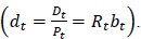 . The variable b
t
is the total amount of public bonds, b
t
= b'
t
+ Ъ''
t
.
. The variable b
t
is the total amount of public bonds, b
t
= b'
t
+ Ъ''
t
.
The primary surplus is given by the difference between the government's total revenue and total expenditure during the same period:

where:


Being
 the government's revenue from household income;
 the government's revenue from taxing the return on physical capital owned by patient households;
 the government's revenue obtained from the total household consumption, and consequently, government consumption is also taxed. Public investment (l
g
) is considered an exogenous shock.
the government's revenue obtained from the total household consumption, and consequently, government consumption is also taxed. Public investment (l
g
) is considered an exogenous shock.
The variable that aims to represent fiscal policy sentiment will be defined in the model based on the fiscal environment. In this case, an increase/decrease in government debt induces a negative/positive polarity in the variable that measures the sentiment of the fiscal authority4. Therefore, the variable that will measure the net negativity of the authority is given by:

If the difference in public debt is positive/negative, we will have higher/lower net negativity, resulting in a more pessimistic/optimistic fiscal policy sentiment; e SFt represents a shock arising from abrupt changes in the fiscal environment.
2.3.2 Monetary Policy
The monetary authority adopts an inflation target and sets the interest rate through a rule proposed by Taylor (1993). As indicated, two versions of the interest rate rule will be considered. A basic version, where the central bank looks only at the lagged interest rate level and deviations in future developments and GDP, which we will call the "basic rule", while in the second version, we include deviations in inflation expectations at horizon t + p from its steady-state level. We will call this version of the instrument rule the extended version. The basic version can be represented by the following expression:

This rule specifies that the current nominal interest rate depends on an inertial or lagged component
 ; the deviation of expected inflation from the target set by the monetary authority; the output gap, represented by the deviation of output from its steady-state value; and, finally, an i.i.d. monetary policy shock, e
R
,
t
. The subscripts p e z are integers that can take any value. The extended version can be represented by:
; the deviation of expected inflation from the target set by the monetary authority; the output gap, represented by the deviation of output from its steady-state value; and, finally, an i.i.d. monetary policy shock, e
R
,
t
. The subscripts p e z are integers that can take any value. The extended version can be represented by:

where S t is the variable that measures fiscal sentiment.
2.4 Bayesian Estimation
In this section, we discuss our methodology for estimating and evaluating the models. The solution of the DSGE model was obtained through a first-order Taylor approximation of the equilibrium conditions around the non-stochastic steady-state value. Given the model solution as a state-space representation and a vector of observable variables, the models were estimated using Bayesian techniques. Specifically, a Metropolis-Hastings algorithm, which is a Markov Chain Monte Carlo (MCMC) method, was employed to obtain the posterior probability distribution of the parameters. Two independent chains were generated, each consisting of 400,000 draws, using the Metropolis-Hastings algorithm. The average acceptance rate across the two chains was approximately 40%, and convergence was assessed using the methods proposed by Brooks and Gelman (1998). The first 180,000 draws were discarded to ensure independence from initial conditions. The statistics of interest were then calculated based on the joint ergodic posterior probability distribution of the structural parameters.
For the estimation, three variables were used for each quarter: real GDP, nominal interest rate, and household consumption. These variables were chosen because they are the most relevant endogenous variables. The variables were used in natural logarithms and seasonally adjusted. The cyclical component of the variables was obtained using the Hodrick-Prescott filter and covers the quarterly period from the first quarter of 2003 to the second quarter of 2021. The model was estimated using Dynare within the Matlab software.
2.5 Calibration and Prior Distributions
Some parameters were fixed during the estimation process, while others were estimated. For the parameters that were kept fixed, we chose to use values from the related literature Christiano and Eichenbaum (1992), Lim and McNelis (2008), Silva, Paes, and Ospina (2014), Cavalcanti et al. (2018), Wesselbaum (2017). Table 5 in Appendix (A) presents a brief description of these parameters.
For the estimated parameters, we opted to use prior distributions similar to those employed in the related literature. For the parameters indicating the degree of substitution between private consumption and the consumption of public goods and services, μ𝑝 e μ𝑖,, we used a prior beta distribution with a mean of 0.50, consistent with the value found for Brazil by Ferreira and Nascimento (2005), Santana, Cavalcanti, and Paes (2012), and Bezerra et al. (2014) 5, with a standard deviation of 0.02 for both. For the parameters of the Taylor rule, we used prior distributions and values for the hyperparameters commonly found in the literature (Smets and Wouters, 2003). The parameter governing the central bank's response to price changes, ϕ π , was set to 1.5, satisfying the Taylor principle. For the coefficient measuring the central bank's response to the output gap, 𝜙𝑌, we used a prior normal distribution with a mean of 0.125 (Carvalho, Silva, and Silva, 2013).
For the parameter indicating the share of physical capital in the production function, similar to Cavalcanti et al. (2018), we adopted a prior normal distribution with a mean of 0.30 and a standard deviation of 0.05. Finally, for all autoregressive parameters, we employed a prior beta distribution with a mean of 0.95 and a standard deviation of 0.02.
3 Results
3.3 Estimations of the Reaction Function
For the estimation of the monetary policy rule, in addition to the traditional variables (interest rate, inflation gap, and output gap) and sentiment indices, other fiscal and fiscal expectations variables were added. The objective of adding these variables is to try to isolate the effects of fiscal communication in the Central Bank's reaction function. The additional variables are:
Government Primary Balance, Government Nominal Balance, Public Debt, Public Debt Cycle, Primary Balance Expectation, Nominal Balance Expectation, Public Debt Expectation.
Table 2 presents the estimations of the Central Bank's reaction function using OLS and GMM. Columns 2 and 3 show the OLS estimates of the reaction function, while columns 4 and 5 present the reaction function estimates obtained using the GMM method. The first includes the fiscal sentiment indices in the reaction function, while the second restricts the interest rate response to variations in the sentiment indices.
As in the work of Silva and Besarria (2018), in general, the results obtained from the estimation of the reaction function, regardless of the method, show a high degree of smoothing in the interest rate dynamics, indicating that the Central Bank makes gradual changes to the interest rate. Regarding the coefficient related to inflation expectations, it is observed that it is statistically significant and greater than one, indicating that the Central Bank satisfies the Taylor principle by increasing the real interest rate in response to deviations in expected inflation.
Table 2 Estimation of the Reaction Function
| Parameters in Structural Form | ||||||||
|---|---|---|---|---|---|---|---|---|
| 𝑶𝑳𝑺𝟏 | 𝑶𝑳𝑺𝟐 | 𝑮𝑴𝑴𝑹 | 𝑮𝑴𝑴𝑰𝑹 | 𝑶𝑳𝑺𝟏 | 𝑶𝑳𝑺𝟐 | 𝑶𝑳𝑺𝑹 | 𝑶𝑳𝑺𝑰𝑹 | |
| 𝑺𝒆𝒍𝒊𝒄𝒕−𝟏 | 0,9371 | 0,8824 | 0,9168 | 0,8412 | 0,9371 | 0,8824 | 0,9168 | 0,8412 |
| [0,0303] | [0,0300] | [0,0228] | [0,0284] | - | - | - | - | |
| Inflation Gap | 0,2569 | 0,2085 | 0,2636 | 0,2289 | 4,0843 | 1,773 | 3,1683 | 1,4414 |
| [0,0385] | [0,0378] | [0,0394] | [0,0398] | - | - | - | - | |
| GDP Gap | 0,0012 | 0,0035 | 0,0031 | 0,0048 | 0.0191 | 0,0102 | 0,0421 | 0,0302 |
| [0,0001] | [0,0001] | [0,0001] | [0,0001] | - | - | - | - | |
| Primary Balance | 0,0811 | 0,1472 | 0,0707 | 0,0971 | 1,2893 | 1,2517 | 0,8498 | 0,6115 |
| [0,0466] | [0,0457] | [0,0466] | [0,0458] | - | - | - | - | |
| Public Debt | -0,0219 | -0,0221 | -0,0237 | -0,0269 | -0,3482 | -0,1879 | -0,2849 | -0,1694 |
| [0,0107] | [0,0115] | [0,0106] | [0,0120] | - | - | - | - | |
| Public Debt Cycle | 0,0017 | 0,0094 | 0,0046 | 0,0111 | 0,027 | 0,0799 | 0,0553 | 0,0669 |
| [0,0121] | [0,0113] | [0,0113] | [0,0120] | - | - | - | - | |
| Primary Balance Expectation | 0,0046 | 0,0018 | -0,0176 | -0,0494 | 0,0731 | 0,0153 | -0,2115 | -0,3111 |
| [0,0653] | [0,0570] | [0,0609] | [0,0570] | - | - | - | - | |
| Nominal Balance Expectation | -0,1172 | -0,0525 | -0,1352 | -0,1129 | -1,8633 | -0,4464 | -1,625 | -0,711 |
| [0,0448] | [0,0432] | [0,0405] | [0,0395] | - | - | - | - | |
| Public Debt Expectation | -0,0191 | -0,0211 | -0,0116 | -0,0038 | -0,3037 | -0,1794 | -0,1394 | -0,0239 |
| Expectation | [0,0117] | [0,0122] | [0,0091] | [0,0111] | - | - | - | - |
| SFF | - | -0,6345 | - | -0,5319 | - | -5,3954 | - | -3,3495 |
| - | [0,3821] | - | [0,4101] | - | - | - | - | |
| SFV | - | 0,7875 | - | 0,6836 | - | 6,6964 | - | 4,3048 |
| - | [0,1936] | - | [0,2020] | - | - | - | - | |
| SFL | - | 0,2087 | - | 0,0889 | - | 1,7747 | - | 0,5599 |
| - | [0,1003] | - | [0,0955] | - | - | - | - | |
Note: The terms in brackets represent the standard deviations of the estimated coefficients.
Regarding the sentiment indices, the OLS and GMM estimates indicate that the SFF variable does not have statistical significance. The SFL variable showed significance only in the OLS model. On the other hand, the SFV sentiment index demonstrated statistical significance in both models, with a positive sign in the models. Thus, when the tone of the National Treasury's communications is optimistic, the Central Bank increases the interest rate, and when the tone is more pessimistic, the monetary authority reduces the interest rate. It is also worth noting that the weight assigned to variations in fiscal policy sentiment was higher than the weight related to inflation expectations.
These results indicate that fiscal policy sentiment significantly affects the conduct of monetary policy, more specifically through the SFV index. It is worth noting that this sentiment index uses public debt as the dependent variable in its construction, while the SFF index relies on a fixed financial dictionary. Therefore, these results make it evident that the fiscal environment (represented by the sentiment index) is a relevant variable in the conduct of monetary policy. Consequently, such results may suggest the possibility of a fiscal dominance scenario. Since the SFV index was constructed based on public debt as the dependent variable, it reflects the market's perception of fiscal sustainability.
If the results show that the SFV significantly influences monetary policy decisions, this may indicate that the central bank is adjusting its policy based on fiscal conditions. In other words, when the SFV reflects fiscal deterioration, the central bank may choose not to raise interest rates, even if inflation is rising, to avoid worsening the government's fiscal situation.
This subordination of monetary policy to fiscal needs is a clear indication of fiscal dominance, where the need to stabilize public finances takes precedence over controlling inflation or other monetary policy goals.
Despite these results, the estimation of simple equations presents some issues. As highlighted by Lubik and Schorfheide (2007), Finocchiaro and Heideken (2013), and Silva and Besarria (2018), these estimations suffer from endogeneity when estimated by OLS and may exhibit bias when estimated by GMM, due to sample size and bias related to the use of stages in two-stage GMM and iterative GMM estimations, which is proportional to the number of moment conditions in instrumental variable models. Moreover, in practice, finding good instruments to implement the GMM method is not trivial. Invalid or weak instruments represent a serious challenge for reliable inference and may compromise the estimates.
3.4 Estimations of DSGE Models
This subsection presents the results of the estimation of the DSGE models. Table 5 (Appendix) shows the mean values, standard deviations, and the corresponding lower (HPD inf) and upper (HPD sup) bounds of the 95% Highest Posterior Density (HPD) credibility interval for the estimated parameters using the Bayesian inference technique for the two types of models estimated.
As found in the work of Silva and Besarria (2018), it is observed that the estimated parameters show little variation between the two models, with posterior means very close between the two. The estimation results reveal that Brazilian data provide little information regarding the amount of labor supplied by patient households in the production of intermediate goods. A similar result was identified by Finocchiaro and Heideken (2013) in their estimations of this parameter for the United Kingdom and Japan, where the posterior mean value was exactly equal to the prior value.
For the parameters defining the maximum borrowing capacity of impatient households and entrepreneurs, the values were lower than the prior mean. These estimates may reflect the fact that households and firms in the country face more restrictive access to credit compared to developed countries.
The parameters for preference and technology shocks were higher than the prior mean, revealing that these shocks are more persistent than initially hypothesized by the prior distribution hyperparameters. Finocchiaro and Heideken (2013) obtain similar results in their estimations of shock processes for the United States, United Kingdom, and Japan.
Regarding the parameters of the Central Bank's reaction function, the parameter measuring the Central Bank's response to changes in inflation expectations was positive and greater than one, satisfying the Taylor principle. Similarly, the parameter measuring the response to output deviations was positive. Both parameters suggest the behavior of a Central Bank operating under a flexible inflation targeting regime, assigning weight to both inflation and the real side of the economy. Regarding fiscal policy sentiment, the mean of the parameter reflecting the Central Bank's response, ф 5 , was positive and significant. Therefore, as in the case of the simple equation models, there are indications that the BCB explicitly considered fiscal policy sentiment, i.e., the fiscal environment, in its reaction function during the period analyzed.
According to Silva and Besarria (2018), a convenient tool in Bayesian analysis is the use of estimates to compare alternative models. One such method is to use the marginal density of the data associated with each model and compare them, subsequently choosing the model best supported by the data. One way to obtain the marginal density of the data, from the joint posterior distribution, is to use Geweke's (1999) estimator, the modified harmonic mean estimator. Table 3 presents the values for the marginal density of the data (in log) computed using this estimator.
Table 3 Comparison Between Models
| Specification | Marginal Data Density | Log Bayes Factor |
|---|---|---|
| Without fiscal policy sentiment | 147.6836 | 0 |
| With fiscal policy sentiment | 220.4311 | 72.7475 |
Note: Own elaboration.
Based on the model evaluation criteria created by Kass and Raftery (1995), we found some evidence in favor of the model that includes fiscal policy sentiment. Therefore, based on the estimations, it can be said that there is evidence, albeit limited, that the BCB explicitly considered fiscal policy behavior in its interest rate decision-making process.
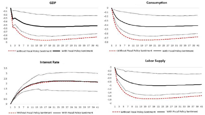
An analysis of the impulse response functions (Appendix B) indicates that the inclusion of fiscal policy sentiment in the reaction function alters the transmission of monetary policy on GDP, household consumption, and labor supply, with the exception of the interest rate. It is also evident that the increase in the interest rate brought typical recessionary effects to the economy, showing that the positive interest rate shock caused a reduction in consumption, labor supply, and aggregate demand. These effects were observed regardless of whether the Central Bank included fiscal policy sentiment in the reaction function or not.
The results obtained from the estimations of the DSGE models, although limited, align with those found in the OLS and GMM model estimations. In other words, the results indicate that fiscal policy sentiment is a relevant variable in the monetary authority's decision-making process regarding the interest rate. Thus, this new investigative approach suggests a high likelihood of the occurrence of the fiscal dominance phenomenon during the analyzed period. These findings converge with those reported in the works of Ázara (2006), Junior, Garcia-Cintado, and Junior (2021), Ornellas and Portugal (2011), and Nobrega, Maia, and Besarria (2020).
4 Conclusion
The recent fiscal situation in Brazil raises the question of whether, and to what extent, the Central Bank of Brazil has reacted to this scenario during the period from 2003 to 2021. This article investigates this issue through two main strategies. The first involves estimating central bank reaction functions using simple equations, including fiscal policy sentiment as one of the arguments in the equation. The second develops a Dynamic Stochastic General Equilibrium (DSGE) model and uses it to produce inferences about the behavior of monetary policy in response to fiscal authority sentiment.
The results suggest that the central bank incorporated the fiscal authority's sentiment into its monetary policy decisions. By reacting positively to the tone of the fiscal authority's communication, the Central Bank of Brazil may have adopted a stance of increasing or decreasing the interest rate when the fiscal outlook was more optimistic or negative, respectively, indicating potential fiscal dominance.
Despite the promising results, future versions need to address certain issues to make the findings more robust. First, constructing a fiscal sentiment variable using Portuguese-language dictionaries could test whether significant changes occur in the results. For future research, it would be worthwhile to use the dictionary by Machado (2019). Another point is that, besides the dictionary by Lima, Godeiro, and Mohsin (2019), there are other dictionaries that use machine learning, so testing these alternatives would also be important to provide greater robustness to the results.
It is also recommended that future research not only test the inclusion of fiscal authority sentiment but also examine fiscal policy uncertainty. In the present study, we discussed whether the sentiment or tone of fiscal policy affects the monetary authority's interest rate decisions, but fiscal policy uncertainty may also play a role-or even more so-than sentiment. Therefore, we recommend including an index of fiscal policy uncertainty, particularly the Macroeconomic Uncertainty Index (IIM) created by Besarria et al. (2021), which is an uncertainty index constructed using Natural Language Processing of the Federal Public Debt Monthly Reports.