


Serviços Personalizados
Journal
Artigo
 Inglês (pdf)
 Artigo em XML
 Referências do artigo
 Enviar este artigo por email
Indicadores
-
 Citado por SciELO
 -
 Acessos
Links relacionados
-
 Citado por Google
 -
 Similares em
SciELO
Similares em
SciELO -
 Similares em Google
Compartilhar

 Permalink
DYNA
versão impressa ISSN 0012-7353versão On-line ISSN 2346-2183
Dyna rev.fac.nac.minas v.79 n.172 Medellín mar./abr. 2012
NUMERICAL TESTS ON PATTERN FORMATION IN 2D HETEROGENEOUS MEDIUMS: AN APPROACH USING THE SCHNAKENBERG MODEL
PRUEBAS NUMERICAS SOBRE LA FORMACION DE PATRONES EN MEDIOS HETEROGENEOS 2D: UNA APROXIMACION A TRAVES DEL MODELO SCHNAKENBERG
DIEGO A. GARZÓN-ALVARADO
Ph.D. National University of Colombia, dagarzona@bt.unal.edu.co
CARLOS GALEANO
M.Sc. National University of Colombia, chgaleanou@unal.edu.co
JUAN MANTILLA
Ph.D. National University of Colombia, jmmantillag@unal.edu.co
Received for review April 2th, 2010, accepted February 1th, 2011, final version Mach, 2th, 2011
ABSTRACT: This paper presents several numerical tests performed on Turing space when spatial parameters in reaction-diffusion equations changes. The tests are performed in 2D on square units in which we perform subdivisions (subdomains). In each subdomain we set parameters that correspond to different wave numbers and therefore presents a heterogeneous medium. Each wave number is predicted by the linear stability theory and correspond to different Turing patterns. The reaction equation chosen is that of Schnakenberg. The results show complex patterns that mix bands and spots, as well as patterns that do not correspond with the original patterns that could be found independently in each subdomain.
KEYWORDS: Reaction-diffusion, Turing instabilities, heterogeneous medium
RESUMEN: Este articulo presenta distintas pruebas numéricas en dominios que presenta variación de parámetros, de forma espacial, de la ecuación de reacción- difusión en el espacio de Turing. Las pruebas son desarrolladas en cuadrados de lado unitario 2D en el cual se realizan subdivisiones (subdominios). En cada subdomminio se ingresan parámetros que corresponden a los diferentes números de onda, por lo tanto presentan un medio heterogéneo. Cada número de onda fue predicho mediante la teoría lineal de estabilidad y corresponde a diferentes patrones de Turing. La ecuación de reacción elegida es Schnakenberg. Los resultados muestran patrones complejos de bandas mixtas y puntos, además, los patrones no corresponden a los patrones originales en cada subdominio.
PALABRAS CLAVE: Reacción-difusión, inestabilidades de Turing, medio heterogéneo
1. INTRODUCTION
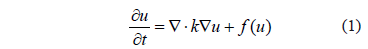
Several physical problems can be modeled by balancing two phenomena: diffusion and reaction [1]. The first is defined as the dispersion of a species involved in a process throughout the physical domain of a problem. On the other hand, reaction is the process of interaction through which the species involved are generated or consumed in the phenomenon. The partial differential equation of reaction-diffusion (RD) for a single species can be written as (1):
where  is the concentration of the substance studied,
  is the diffusion constant and
  is the function that defines the reaction process. This equation and other more complex models of RD systems, where more species or reactants are involved, have the ability to create spatial-temporal patterns. A particular case is called Turing instability [1,7] which is characterized by creating stable patterns over time and unstable in space. Due to this, RD systems have been used to study problems in areas such as fluid dynamics [2], heat transfer [3], semiconductor physics [4], materials engineering [5], chemistry [6], biology [7], population dynamics [8], astrophysics [9], biomedical engineering [10] and financial mathematics among others. It should be noted that equation (1) requires appropriate boundary conditions [11].
Thanks to experimental and theoretical studies on RD systems, the knowledge of it has been steadily growing [12-13] and, in turn, new models have been proposed that involve, in their simplest form, two chemical species [14]. Reaction-diffusion systems have been classified into three categories which are: (a) systems based on real reactions [14] (as is the case of the Thomas reaction), (b) Reaction-diffusion systems based on hypothetical reactions (e.g., the Schnakenberg reagent system), and (c) systems that emulate patterns found in nature (eg Gierer Meinhardt's reaction). These types of RD systems have in common that spatial patterns can be stable over time if the parameters of the reactive terms and diffusion constants are in a well-defined space called the Turing space [1].
Therefore, an RD system, of two species, is defined by (2):
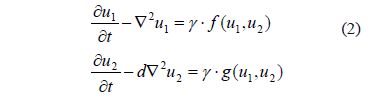
Spatial instability will be present in the patterns of concentration of species  and
and  if each of the conditions imposed (which define the Turing space) are fulfilled in (3) [28].
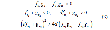
where and
and  indicate the derivatives of the reaction functions with respect to the concentration variables, for example
 . In expressions (1) and (2)
  is the ratio of diffusion coefficients of the two species
  and
and  ; furthermore, in (2)
  is a undimensional coefficient associated with the reactive processes
 and
and  [1,15].
The analysis of these RD systems, which have Turing instability has been developed from two frameworks: by mathematical analysis [1] and through numerical simulation [1,15]. From the analytical standpoint, efforts to understand the behavior of RD systems have focused on the study of the relationship between branches of the space parameter and pattern formation. In this approach, RD systems have been studied by the comparisons of sub and super solutions, degree theory, the Conley index, the theory of critical dots, and singular perturbations for various types of principal maxima [11]. These methods have been effective for the analysis of stationary solutions and traveling waves [16]. Also, there are studies on complex branching scenarios in RD systems by applying methods of the group theory for problems with symmetries [17]. Efforts in this area of mathematical analysis and specifically, systems dynamics, have allowed for the construction of knowledge that has been tested and extended from the stand point of numerical simulation.
The numerical simulation of RD systems has confirmed the existing knowledge about pattern formation. For example, Madzvamuse et al. [7,15], Painter et al. [17,18] have developed numerical examples of pattern formation in the two-dimensional domain under the growth action of the domain. In Madvamuse [15], numerical simulations are developed using a Lagrangian scheme with a moving mesh. These simulations show a large difference between the steady state for fixed domains and the continuous formation of new patterns for growing domains. In [15] the appearance of different structures that can vary among band systems, dots, and combinations of these domains with decreasing exponential growth is reported. Madzvamuse [19] reported the formation of patterns in the presence of convective fields with null divergence. In turn, from a numerical point of view, we have studied the effects of fields on the formation of convective patterns. Garzón-Alvarado et al. [20] show the pattern formation and transition of a Turing patterns to traveling waves in the presence of toroidal velocity fields that change the dynamics of the system. There are also studies on other phenomena in the generation of Turing patterns such as, for example, the heterogeneity of the reagent parameters that cause complex patterns in the solution of the RD systems [14,21]. Voroney et al. [21] show the interaction between oscillatory dynamics and pattern formation when heterogeneous parameters are presented in space, in this case a solution exists using the Sel'kov reagent system.
Following the study of heterogeneities in space and under the numerical approach, the objective of this paper is to computationally solve the 2D RD equations for the Schnakenberg reaction system, in domains with non-homogeneous kinetic parameters, leading to uniform steady states that vary in the spatial domain. This paper gives a solution to the RD equations system using the finite element method with the evaluation of the nonlinear terms in the new time step, thus adopting the Newton-Raphson method. In this paper we developed some numerical examples that allow us to observe how the spatial variation in the parameters of the RD equations generates complex Turing patterns.
The paper is organized as follows: first, it shows the mathematical model of reaction-diffusion system, especially in this article we used the Schnakenberg model. In addition, this section illustrates the theory on the prediction of wave numbers in different Turing spaces. Then it shows the finite element formulation for solving the RD system. In the next section we present examples to solve the boundary conditions, the type of domain and computational parameters. Later it shows simulation results and ends with discussion and conclusions from the patterns obtained.
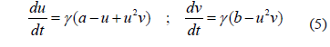
2. THE REACTION MODEL: SCHNAKENBERG MODEL
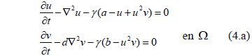
The RD system in (2) can be written, for the case of the Schnakenberg reagent model [1,15,19], as (4):
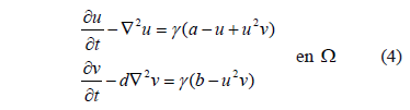
where u and v are the chemical species,  and
and  the diffusive terms and
 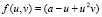 and
and  the reagent terms. Moreover, g is a dimensionless constant a and b are constant parameters of the model. We have imposed homogeneous Neumann conditions and initial conditions are small perturbations around the homogeneous steady state of each of the reactive terms, this is,
  and
and  .
.
2.1. Conditions for the diffusion instability
From Murray [22] we can establish that without the presence of the diffusive term, u and v must satisfy (5):
For small perturbations around the steady state  (this is
 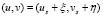 ), equation (5) is linearized as (6):
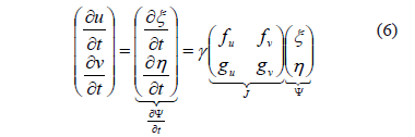
where ,  , and
, and  . In (6), we have conducted a expansion in series where we have neglected terms of order greater than 2. It should be noted that
  and
and  are evaluated in the steady state
 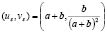 .
.
A solution to (6) can be written as (7):
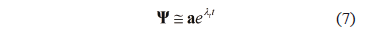
where  is a vector containing information fo the initial conditions. Replacing (7) in (6) we obtain (8):
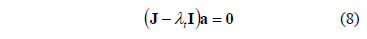
where  is the identity matrix. For there to be a nontrivial solution it requires that
  , so we get the following characteristic Eq. (9):

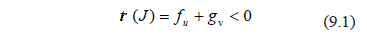
Then (6) is linearly stable if and only if the conditions are fulfilled (9) for which the real part of the eigenvalues  are negative. Note that these conditions are analogous to Routh-Hurwitz [22]:
If the diffusive term is introduced we get the linear differential equation (10):
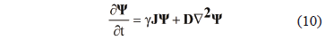
with  . Using the homogeneous boundary conditions (
 ), equation (10) can be solved by separation of variables, with
  , so you can get a solution by the form (11):
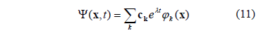
where  is the wave number of the spatial pattern or eigenvalue described in [15],
  is the vector of Fourier coefficients and
 is the eigenfunction of the Laplacian (with
 ) given by (12):

Replacing (11) in (10) yields:
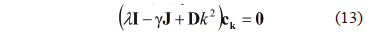
where  is the vector of zeros and
  is the identity matrix. As in the case of the differential equation without diffusion, requires that the vector of Fourier coefficients is not trivial, so we must verify the following condition:

With what we get the dispersion relation (or characteristic equation from (13)) [1,15,22] (15):
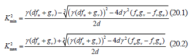
Therefore, for Turing instability occurs, the roots of (15.1) must satisfy for some  . According to Ruth-Hurwitz conditions [22], so that the real part of the eigenvalues be positive it is required that
  and
and  , or vice versa. From the condition (9.1) we can conclude that
  for all
  .Therefore, it is required that
  .
.
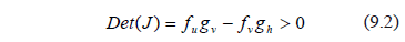
In (15.3) we can see that  and by (9.2) we know that
 , therefore, it must be satisfied that, which it is a necessary condition, but not sufficient. The additional relation is found by minimizing
  where it must meet
  . This is done by , where we get (16):

Replacing (16) in (15.3) yields (17):
From where we obtain the last condition for Turing instability. Reorganizing the conditions to be met we obtain, in summary, the following inequalities (18):

2.1.1. Definition of the wave number
At that point where  , we get a bifurcation parameter [1,15]. Therefore, from (18.4) we have that
  determines the bifurcation point, for a value
 , called critical diffusion coefficient, above which Turing instabilities are obtained. Therefore, the critical value of diffusion
  is given by (19):

On the other hand, having  we get the value for
  for which there is a range of possible wave numbers, only if
  . This is shown in Fig. 1.
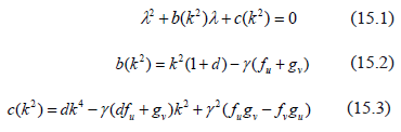
Figure 1. Graphics for . Each of the curves are drawn for the Schnakenberg reaction model with
  ,
,  and
and  . Previously, using Eq. (19) we had found that
Using  and replacing its value in
  (equation (15.3) we obtain the red curve. The magenta curve is obtained by
  , and the green curve is obtained for
  . In the graph
 and
and

As shown in Fig. 1, if  is satisfied, at the cutoff point of
  with the axis
 (this is where the dots are
  ) we obtain two important points wich are
  and
and  . These points define a range where we find the wave numbers or eigenvalues that will present the solution of the RD system. These values are given by:
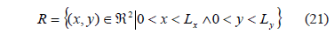
This interval  defines the wave number of the RD system solution in a Turing space. To define the behavior of the instability we must define the domain over which the solution takes place. In [1,15] is solved on a square, but for generality, we will provide information about a rectangle.
2.1.2. Eigenfunctions of a rectangle
Consider the rectangle whose length of each side in the direction of  and
and  is
is  and
and  , respectively [1,15]:
In [15] we can verify that the eigenfunctions for the equation (11) are given by (22):
Whose eigenvalues are in the shape of:

When  , the solution of the linearized system (10) is:
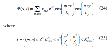
For example, in the case shown for Fig. 1, with  ,
,  ,
,  and
and  , have that
 and
and  . Then in a unit square (
 ), the interval is given by (
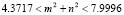 ). Then we must choose
  and
and  integers that satisfy the whole range proposed. In this case the values are
  and
and , or vice versa. In conclusion, the wave number is
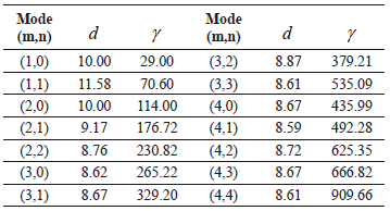
  . Following a similar analysis yields Table 1 [15] where we observe the wave numbers and values for
 and
and  with constant values
 and
and  .
.
Table 1. Modes of vibration for for different values of
  and
and  of the Schnakenberg model [15]
2.2. Finite element solution
To solve the system of equations (4) we have chosen the finite element method. We have also used the Newton-Raphson method to solve the nonlinear problem that evolves over time. The time integration has been made using the trapezoidal rule. Then, u and v must be found by its correct interpolation with the shape functions given in [23]. To carry out the exhibition we start with the weak formulation of the problem and follow a procedure similar to that used in [24].
2.2.1. Weak formulation
Be (4) rewritten as:
Consider the equation (4.a) is sufficiently smooth and differentiable. Using Gauss's theorem we can prove that (26):
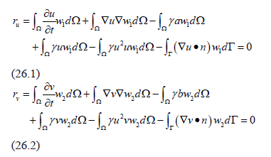
where  and
and  are weighting functions and
  is the normal vector directed outwards from the dominion
  over the frontier
 . Keep in mind that it must be impose homogeneous Neumann boundary conditions so that the last term of equations (5.1) and (5.2) disappear.
To move to the discrete solution, the variables are written in terms of nodal values using the weighting functions as [23]:

where  and
and  are the shape functions that depend only on space,
  and
and  are the values of u and v at the nodal points and the superscript h indicates the discretization of the finite element variable. By substitution of (26) in (25) and the choice of weighting functions equal to the shape functions we obtain residue vectors of the Newton-Raphson method given by [22] (28):
where  and
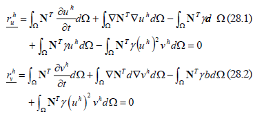
and  are the residue vectors that are calculated at the new time. Meanwhile, each of the positions (inputs) of the Jacobian matrix are given by (29):
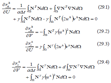
where  is a feature parameter of the temporal integration method [23] and
 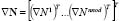 is the row vector of the first spatial derivatives of the shape functions. In this case we used bilinear elements of 4 nodes as described in [23].
2.3. Numerical tests
To solve the system of equations resulting from the finite element method with Newton-Raphson method we created a program in FORTRAN and resolved all the examples illustrated below in a Laptop of 4096 MB RAM and 800 MHz speed processor.
The mesh used is the same for all examples, which has 2500 bilinear regular elements of 4 nodes each, for a total of 2601 nodes.
Moreover, the initial conditions are the same for all the examples, with small random perturbations of 10% around the steady state [15].
Numerical solutions over homogeneous domains (control)
Initially we solved the system given in (4) for completely homogeneous domains in order to have a frame of reference and comparison for all subsequent numerical tests.
Figure 2 shows the results for the variable u of the Schnakenberg equation. Note the formation of dot patterns (cases b, d, e, g, h, i, k, l, n) and rows (a, c, f, j, m). Special attention deserves the case m) where we have with two possibilities for Turing pattern formation given by the dynamics of the system, which can choose among forming a wave number  , or, a pattern by the type
  . By the principle of minimum energy, in this case the pattern
  was formed.
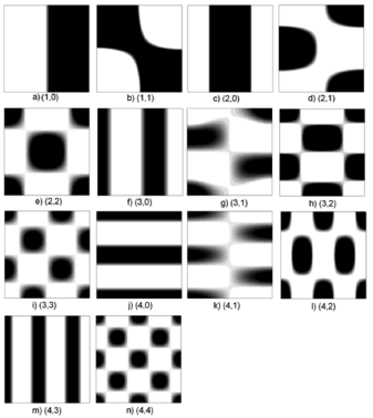
Figure 2. Turing Patterns in steady state for different wave numbers.
a(1,0); (b) (1,1); (c) (2,0); (d) (2,1); (e) (2,2); (f) (3,0); (g) (3,1); (h) (3,2); (i) (3,3); (j) (4,0); (k) (4,1); (l) (4,2); (m) (4,3); (n) (4,4).
For further reference see Table 1. The black color has concentration values higher than 1.0. Black color: high concentration, White color: low concentration. The figure has been made for the concentration u in Eq. (4).
The wave number indicates the number of half sine waves in each of the directions x and y. Figure 3 provides an explanation for a wave number (4,2), which notes 4 half-waves in x direction and 2 half waves in y direction.
Figure 3. Explanation of the correspondence of the wave number and Turing pattern for a (4,2) value.
2.3.2. Heterogeneous domains, subdomains location
To observe the independence of the location of the subdomains in the formation of Turing patterns we carried out several numerical tests as (see Fig. 4): Divide the domain into two subdomains, where in each one of them their respective parameter is taken according to the specific wave number given in Table 1. Example: Figure 4(a) shows two sub-domains (upper and lower). In the lower subdomain we have chosen the parameters  and
and  corresponding to a wave number
 and at the upper level domain we took
  and
and  which generates a mode in the shape of
  . Figure 4(b), (c) and (d) show the different subdomains that have been tested.
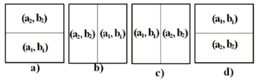
Figure 4. Types of subdomains chosen for the test of independence of the location of the different modes.
We show, only the results of Fig. 5, where the wave modes that have been chosen are  and
and  . It should be noted that the initial conditions do not change between each of the examples, so that each temporary path to the steady state is different. Then we have different spatial patterns in times
  and
and  . In
. In  we have the same type of pattern, in each of the examples but with a 90° rotation, as expected if the initial conditions do not affect the steady-state results.
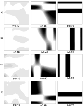
Figure 5. Numerical examples for a heterogeneous domain with  and
and  . (a), (b), (c) and (d) according to the distribution of subdomains given in Fig. 4(a), (b), (c) and (d), respectively. At the bottom it shows the time during the transient simulation to reach steady state in
  .
.
2.3.3. Heterogeneous domains: numerical test for and
and  given in Table 1 (Fig. 6).
Using the configuration (b) of Fig. 4, numerical test are made where  and
and  are different wave numbers given in Table 1. Figure 6 shows the results of the numerical experiment.
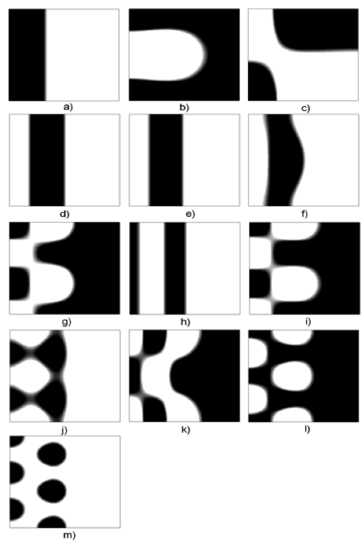
Figure 6. Turing patterns in steady state for two heterogeneous medium with different numbers given by  and given by:
(a) (1,1); (b) (2,0); (c) (2,1); (d) (2,2); (e) (3,0); (f) (3,1); (g) (3,2); (h) (3,3); (i) (4,0); (j) (4,1); k) (4,2); l) (4,3); m) (4,4).
It is noted that the final patterns (steady state) have a certain complexity with respect to those in Fig. 2. In case (a) shows that the wave number (1,0) is in the left subdomain. This wave mode dominates and silences the mode (1,1) so at the end the result is "similar" to a mode (1,0) where low density values are dominant in 75% of the domain. In case (b) gives a result that is not similar to any of the modes of the subdomains. Here we see a "drop" of low concentration found in 70% of the domain. In c) shows the simulation for the wave numbers (2,1) and (1,0). For this case the ending result is similar to a wave number with a value of (1,1) not symmetric. Cases (d), (e) and (f) show similar patterns. The wave numbers of the subdomains are (1,0) with (2,2) (3,0) and (3,1), respectively. In the f) case it shows a pattern with a strip with a horizontal excitation (curve), which can be explained by the high excitation of the wave number (3,1). In cases (g) and (i) shows the numerical results with subdomains with wave numbers (3,2) and (4,0), respectively. It is noted that the results are similar for these two cases. We can see that half of the domain has a high concentration of u. The left half has a vertical "pseudo-mode" of 3. On the left side we can see the formation of dots, while on the right side we notice a block of high density of u with an edge that has saw-tooth shape. In the( h) case, with wave modes (1,0) and (3,3), show the formation of a "pseudo-mode" wave of (3,0) (bands), where the last half wave (right side) is very elongated (see Fig. 2). In (j) shows the simulation with wave numbers (4,1) and (1,0). It is noted that the left side generates a "pseudo-mode" in the vertical direction of 4. In the horizontal direction we can not set one only mode. There is a distorted dot pattern similar to a semicircular sector. Case (k) shows a pattern for wave numbers (1,0) and (4,2). This pattern is similar to that found in (g) and (i), however, the left side is a pseudo mode in the vertical direction of 2. The right side shows a single saw tooth. In (1) the formation of dot patterns (low concentration of u with modes (1,0) and (4,3)) is shown without symmetry, these dots are elongated horizontally. In the vertical direction we have a pseudo-mode of 4 in the left side. In (m) it shows the formation of dots of high concentration.
2.3.4. Heterogeneous Domains: Numerical test for  and
and  given in Table 1 (Fig. 7).
Using a configuration similar to the previous case we did numerical tests with  and
and given in Table 1. Fig. 7 shows the results of the numerical experiment.
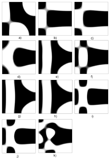
Figure 7. Turing patterns in steady state for two heterogeneous medium with different numbers given by  and
and  given by:
(a) (2,1); (b) (2,2); (c) (3,0); (d) (3,1); (e) (3,2); (f) (3,3); (g) (4,0); (h) (4,1); (i) (4,2); (j) (4,3); (k) (4,4).
Again we observe the difference between the original Turing patterns and the new patterns formed by heterogeneous medium (Fig. 7). Figure 7(a) shows the result for modes with each subdomain (2,0) and (2,1). Note the formation of a pattern similar to a vibration mode (2,1) where we have invested the maximum value of the variable u that is shown in Fig. 2(d).
Figure 7(b) and (c) show similar results. We observe the formation of a band of great length on the right side and two dots on the left. In the vertical direction appears a vibrating pseudo mode of 2, while in the horizontal direction there is a pseudo-mode of 1. Note that the resulting pattern is symmetrical with respect to the axis y=0.5 but does not preserve the original symmetry. The original modes (in each subdomain) are (2,0) and (2,2) and (3,0) for b) and c) respectively. In addition, Fig. 8(d) with modes (2,0) and (3,1) has a similar behavior, where the vast band of the right has an appearance like a water drop shape. Figure 7(e), (g) and (h) show the formation of a pattern with dots of low concentration of u on the right side and lines in the left side. The original patterns are (2,0) and (3,2), (4,0) and (4,1), respectively. Note that the vibrating pseudo-mode in the horizontal direction in the center is 2 and on the top and bottom 3, while in the vertical direction is 0 in the left region and 2 on the right.
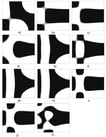
Figure 8. Turing patterns in steady state for two heterogeneous medium with different numbers given by  and
and  given (a) (2,2); (b) (3,0); (c) (3,1); (d) (3,2); (e) (3,3); (f) (4,0); (g) (4,1); (h) (4,2); (i) (4,3); (j) (4,4).
Figure 7(f), (i) and (j) show the patterns developed for subdomains with wave numbers (2,0) and (3,3), (4,2) and (4,3), respectively. There is a symmetrical pattern with respect to  . Again, it presents a band on the right side and three dots on the left side. Note the similarity with Fig. 7(b) and (c). Unlike the latter, there is a pseudo mode of vibration in x and y of 2. The last Fig. 7(k) shows a complex figure which has a combination of dots and bands without symmetry.
2.3.5. Heterogeneous domains: Numerical test for  and
and  given in Table 1 (Fig. 8)
In this case (results in Fig. 8) we used a vibration mode (2,1). The configuration used for the numerical test is similar to that given in previous examples. Figure 8(a) and Fig. 8(b) show the test results for a subdomain (2,1) and (2,2) and (3,0), respectively. Note a similar pattern to Fig. 2(e) being a pseudo-mode (2,2) without symmetry. Note that there is a pattern of dots with the length of these on the right side.
In Fig. 8(c), a pseudo mode (2,2) where the main dot has been separated and has been directed toward the left side of the domain is shown. Note the similarity with a) and b). Figure 8(d) and (f) show the formation of band patterns from a domain with vibration modes (2,1) and (3,2) and (4,0), respectively. The resulting pseudo-mode is (3,0). Figure 8(e) shows the formation of patterns from modes with each subdomain (2,1) and (3,3). We observe in the left side the formation of a figure similar to a "nut" and in the right side the formation of two dots at the top and bottom of the domain. Figure 8(g) shows the dot formation ("water drops") of different sizes that are directed toward the center. It is symmetrical to the axis y = 0.5. Figures 8(h) and (i) are taken as the original modes (2,1) and (4,2) and (4.3), respectively. We observe the formation of a pattern of dots with a pseudo-mode of (3,2). In (j) we observe the formation of a pattern of lines with a pseudo-mode (4,0).
3. CONCLUSIONS
This article has shown many numerical tests where we give evidence that the patterns obtained in a heterogeneous medium present, in general, complex Turing instabilities. In two dimensions there is the possibility of the emergence of mixed patterns of dots and bands. Additionally, they can have complex pseudo-modes wave that can change the length and shape of the bands and dots.
It is also observed, in the case of two subdomains, that the resulting wave mode, in general, is an intermedium mode between the original modes of each subdomain.
Furthermore, the combination of distant wave modes, for example (2,0) and (4,4) presents complex instabilities that do not have a defined wave pseudo-mode, so the symmetry seen in the original patterns is lost.
REFERENCES
[1] Garzón, D., Simulación de procesos de reacción-difusión: Aplicación a la morfogénesis del tejido óseo, Ph.D. Thesis. Universidad de Zaragoza. 2007. [ Links ]
[2] D. White. The planforms and onset of convection with a temperature dependent viscosity, J. Fluid Mech, Vol. 191, pp. 247–286, 1988 [ Links ]
[3] Hirayama, O. and Takaki, R., Thermal convection of a fluid with temperature-dependent viscosity. Fluid Dynamics Research, Vol. 12-1, pp. 35-47, 1988. [ Links ]
[4] Balkarei, Y., GrigorYants, A., Rhzanov, Y. and Elinson, M., Regenerative oscillations, spatial-temporal single pulses and static inhomogeneous structures in optically bistable semiconductors, Opt. Commun. Vol. 66. pp. 161–166, 1988. [ Links ]
[5] Krinsky, V.I., Self-organisation: Auto-Waves and structures far from equilibrium, Ed. Springer, 1984. [ Links ]
[6] Zhang, L. and Liu, S., Stability and pattern formation in a coupled arbitrary order of autocatalysis system, Applied Mathematical Modelling. Vol. 33. pp. 884–896, 2009. [ Links ]
[7] Madzvamuse, A., Wathen, A. and Maini, P., A moving grid finite element method applied to a model biological pattern generator, Journal of Computational Physics. Vol. 190. pp. 478–500, 2003. [ Links ]
[8] Baurmanna, M., Gross, T. and Feudel, U., Instabilities in spatially extended predator–prey systems: Spatio-temporal patterns in the neighborhood of Turing–Hopf bifurcations, Journal of Theoretical Biology. Vol. 245. pp. 220–229, 2007. [ Links ]
[9] Nozakura, T. and Ikeuchi, S., Formation of dissipative structures in galaxies, Astrophys. J. Vol. 279. pp. 40–52, 1984. [ Links ]
[10] Madzvamuse, A., A Numerical Approach to the Study of Spatial Pattern Formation in the Ligaments of Arcoid Bivalves, Bulletin of Mathematical Biology, Vol 64. pp. 501–530, 2002. [ Links ]
[11] Mei, Z. Numerical Bifurcation Analysis for reaction-diffusion equations. Springer Verlag. Alemania. 2000. [ Links ]
[12] Castets, V., Dulos, E., Boissonade, J. and De Kepper, P., Experimental evidence of a sustained standing Turing-type nonequilibrium chemical pattern. Phys. Rev. Lett. 64 24, pp. 2953–2956, 1990. [ Links ]
[13] Maini, P.K., Using mathematical models to help understand biological pattern formation. Comptes Rendus Biologies, Volume 327, Issue 3, March, pp. 225-234, 2004. [ Links ]
[14] Page, K. M., Maini, P. K., Monk ,N. A.M., Complex pattern formation in reaction–diffusion systems with spatially varying parameters. Physica D: Nonlinear Phenomena, Volume 202, Issues 1-2, 1 March, pp. 95-115, 2005. [ Links ]
[15] Madvamuse, A., A numerical approach to the study of spatial pattern formation. D.Phil. Thesis. Oxford University. UK. 2000. [ Links ]
[16] Sagués, F., Míguez, D. G., Nicola, E. M., Muñuzuri, A. P., Casademunt, J. and Kramer L., Travelling-stripe forcing of Turing patterns. Physica D: Nonlinear Phenomena, Volume 199, Issues 1-2, pp. 235-242. 2004 [ Links ]
[17] Painter, K.J., Othmer, H.G. and Maini, P.K., Stripe formation in juvenile Pomacanthus via chemotactic response to a reaction-diffusion mechanism. Proceedings of National Academy Sciences USA, 96, pp.55495554. 1999. [ Links ]
[18] Painter, K.J., Maini, P.K. and Othmer, H.G., A chemotactic model for the advance and retreat of the primitive streak in avian development. Bulletin of Mathematical Biology, 62, pp. 501-525, 2000. [ Links ]
[19] Madzvamuse, A., Turing instability conditions for growing domains with divergence free mesh velocity. Nonlinear Analysis: Theory, Methods & Applications, Volume 71, Issue 12, 15 December, Pages e2250-e2257. 2009 [ Links ]
[20] Garzón-Alvarado, D.A., Galeano, C. y Mantilla, J.M., Experimentos Numéricos sobre ecuaciones de reacción convección difusión con divergencia nula del campo de velocidad. Revista Internacional de Métodos Numéricos en Ingeniería. Aceptado. [ Links ]
[21] Voroney, J. P., Lawniczak, A. T. and Kapral, R., Turing pattern formation in heterogenous media. Physica D: Nonlinear Phenomena, Volume 99, Issues 2-3, 15 December, pp. 303-317, 1996. [ Links ]
[22] Murray, J.D., Mathematical Biology: I. An Introduction (Interdisciplinary Applied Mathematics). Springer Verlag. New York. 1993. [ Links ]
[23] Hughes. T.J.R., The Finite Element Method (linear Static And Dynamic Finite Element Analysis). Dover. U.S.A. 2000. [ Links ]
[24] Javierre, E., Moreo, P., Doblaré, M. and García-Aznar, J.M., Numerical modeling of a mechano-chemical theory for wound contraction analysis. International journal of solids and structures. vol. 46, No. 20, pp. 3597-3606, 2009. [ Links ]

