EXAMPLES IN THE CLASSROOM: PATTERN CLASSIFICATION USING THE R LANGUAGE

EJEMPLOS EN EL AULA DE CLASE: CLASIFICACIÓN DE PATRONES USANDO EL LENGUAJE R

 

JUAN DAVID VELÁSQUEZ HENAO
Ph.D,Universidad Nacional de Colombia, jdvelasq@unal.edu.co

JOHN WILLIAN BRANCH BEDOYA
Ph.D, Universidad Nacional de Colombia, jwbranch@unal.edu.co

 

Received for review: October 10^th, 2011, accepted: February 06^th, 2012, final version: March 26^th, 2012

 

---

ABSTRACT: In many courses with a strong mathematical background, students often experience difficulties when concepts are put into practice to solve problems. In our teaching experience, the R language for statistical computing is a powerful tool for exemplifying algorithms, solving numerical problems, and illustrating concepts by using complex graphics. This paper presents some non-trivial examples of the application of the R language from our instruction of the pattern classification course in our school of engineering.

KEYWORDS: computer graphics, teaching, algorithms, pattern recognition.

RESUMEN: En muchos cursos con un fuerte contenido matemático, los estudiantes usualmente experimentan dificultades cuando los conceptos son puestos en práctica para resolver problemas. En nuestra experiencia docente, el lenguaje R para la computación estadística es una poderosa herramienta para ejemplificar algoritmos, resolver problemas numéricos y para ilustrar conceptos usando gráficos complejos En este artículo, se presentan algunos ejemplos no triviales de la aplicación del lenguaje R en la enseñanza del curso de clasificación de patrones en nuestra facultad de ingeniería.

PALABRAS CLAVE: gráficos por computador, enseñanza, algoritmos, reconocimiento de patrones.

---

 

1. INTRODUCTION

There is a significant trend towards the use of computational tools in the teaching of courses with significant mathematical content; these tools promote learning, motivate students in a different way, and help students to develop practical skills. Examples of these tools are: The Geometer's Sketchpad [1,2] and Cabri Geometry II [3] in the field of geometry, Mathematica [4] and Maple in the area of computer algebra, and Matlab in the field of numerical computation (mostly in engineering).

Moreover, in the teaching of courses in the area of computational intelligence such as

• Artificial neural networks
• Fuzzy and neuro-fuzzy systems
• Pattern recognition and pattern classification
• Statistical learning
• Evolutionary computing
• Swarm intelligence, and
• Bio-inspired algorithms,

the instructor needs to illustrate algorithms, solve numerical problems, and explain concepts and examples using complex graphics. In addition, it is necessary to do practical work with the aim of getting deeper into the concepts presented and to develop specific skills.

This problem is common to the teaching of many academic courses in mathematics, engineering, and economics, and the successful incorporation of computational tools as an integral part of the teaching strategy has been reported. For example, Gorjanc [5,6] presents specific examples of the application of Mathematica in the teaching of geometry in the curriculum of a civil engineering program, and describes the benefits of using this computational tool. Balkin [7] discusses the experiences on the use of Mathematica in the classroom and offers some lessons from their experience in order to improve teaching. Allenby and Rossi [8] describe their teaching experiences and the benefits perceived by students in teaching Bayesian statistics in a doctoral program in business.

The R programming language for statistical computing is an environment, originally developed by Ihaka and Gentleman [9], which implements a programming language that is a clone of the S language developed at AT&T Laboratories [10–12] and S-Plus (which is the commercial version of S); S is a language designed specifically for data visualization and exploration, statistical modeling, and programming with data [13]. The R language is commonly used for teaching and researching in the fields of statistics, forecasting, and econometrics; however, it is almost completely unknown in the academic and research community dedicated to computational intelligence. The first objective of this paper is to contribute to the popularization of R inside of the computational intelligence community.

In our academic experience, we found that the R language is suitable for teaching some courses in the area of computational intelligence due to its characteristics, particularly in teaching a pattern classification and recognition course. The second objective of this paper is to present specific examples of the use of the R language for illustrating algorithms and for building complex graphics.

This paper is organized as follows: In Section 2, we present a short introduction to the R language. In Section 3, several examples are presented. Finally, we conclude in Section 4.

2. The R programming environment and their language

The R environment is a free software under the GNU license given by the Free Software Foundation, which can be downloaded directly from the site http://www.r-project.org/.

Advanced users can interact with the system through a command line, but several packages provide the environment with a graphical user interface based on menus and dialog boxes [14,15].

The programming language is based heavily on the paradigms of functional programming and object-oriented programming [16,17], although it has some similarity with the syntax of the C and C++ languages [18].

Some language features are as follows:

• Mechanisms for handling large amounts of information
• An extensive collection of statistical tools for data analysis
• A system for creating and manipulating complex graphics
• More than 2000 packages to extend the functionality of the environment
• An elegant, simple, and effective programming language
• A system for debugging and exception handling

Several studies have demonstrated the versatility of the R language. For example, the main routines of the R language for the analysis and time series prediction in energy markets are described in [19]; in [20], the implementation of a linear associative memory (a type of artificial neural network) is discussed.

 

3. EXAMPLES

In this section, we present some non-trivial cases on the preparation of examples in the area of pattern recognition and classification using the R language.

3.1. 3-D Surfaces
The plotting of surfaces in three dimensions (3-D) is one of the main tasks performed in the exemplification of many problems in the fields of pattern recognition [21], artificial neural networks [21], and neuro-fuzzy systems [22]. While the R language has several primitive functions for visualizing datasets of two variables in 3-D, there is no function that can build this type of graphic directly for a function. In this first example, we write and use a new function called surface.3D. This new function has the following parameters: the function to be plotted, limits for the and axes, and plots for the resulting 3-D surface. The code of the Surface.3D function is listed in the Appendix. A typical example of the function usage is presented below, and the plot of the function is presented the in Fig. 1.

> bowl <-
+ function(x , y)
+ {
+ cx1 = 1.5
+ cy1 = -1.0
+ z1 = 1/(1 + 2 * (x - cx1)^2 + (y - cy1)^2)
+ cx2 = -1.0
+ cy2 = 1.5
+ z2 = 1/(1 + (x - cx2)^2 + (y - cy2)^2)
+ return( -(z1 + 0.6 * z2) + 5)
+ }
>
> surface.3D( fn = bowl, xlim = c(-3, 3),
+ ylim = c(-3, 3), N = 40, theta = -25,
+ phi = 35, col = 'gray', ltheta = -120,
+ shade = 0.45)
>

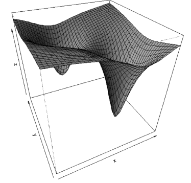
Figure 1. 3-D plot obtained using the surface.3D function

3.2. Bayesian classifier for normal distribution
The fundamental problem addressed in the area of pattern classification is determining to which class, , belongs an element . Depending on the assumptions made about the problem, different methodologies are used for answering this question.

In the simplest case, it is assumed [23]: firstly, that there are only two classes; and secondly, that the probability of the membership of to each class follows a multivariate normal distribution whose parameters are known. The classification rule is expressed using a discriminant function that measures the probability of . Thus, the classification rule can be expressed as:

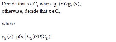
As a first numerical problem, we want to find the decision boundary for the presented case. That is, the point at which g1 (x)=g2 (x), when g1 (x)=p(x|C1) P(C1)=0.3x N [-0.5,1] and g2 (x)=p (x|C2) P(C2)=0.7xN[0.5,1]. The notation N [c,s] represents a normal probability distribution centered at c and with standard deviation s.

To solve the problem, the function [g1 (x)-g2 (x)]2 is minimized numerically using the optim function, which is implemented in the R language distribution. The decision boundary corresponds to the vertical line in Fig. 2(a). The code used to perform calculations and generate Fig. 2(a) is as follows:

> par(mfrow = c(2,1))
> PC1 = 0.3
> PC2 = 0.7
> zz1 = function (x){PC1 * dnorm(x, -0.5, 1.0)}
> zz2 = function (x){PC2 * dnorm(x, +0.5, 1.0)}
> zz3 = function (x) { (zz1(x) - zz2(x))^2 }
> s0 = optim(par = 0, fn = zz3, method =
+ "L-BFGS-B", lower = -3, upper = 3)$par
> curve( expr = zz2, from = -4, to = 4,
+ lwd = 2, ylab = '')
> curve( expr = zz1, from = -4, to = 4, lwd = 2,
+ add = TRUE)
> abline(h=0,lty=3)
> abline(v=0,lty=3)
> text(x=-2.8, y=0.09,
+ expression(p(x/C[1])*P(C[1])))
> text(x=+2.6, y=0.23,+
+ expression(p(x/C[2])*P(C[2])))
> segments(x0=s0, y0=0.0, x1=s0, y1=zz1(s0), lwd=5)
> title(main = '(a)')
>

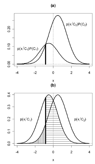
Figure 2. Example of a Gaussian classifier: (a) decision boundary, (b) classification error regions

A related concept is the probability of error when making a decision, which can be expressed as:

For the numerical example presented, the error probability corresponds to the shaded areas in Fig. 2(b), which were obtained with the following code:

> zz4 = function (x){dnorm(x, -0.5, 1.0)}
> zz5 = function (x){dnorm(x, +0.5, 1.0)}
> curve( expr = zz4, from = -4, to = 4,
+ lwd = 2, ylab = '')
> curve( expr =zz5, from= -4, to = 4, lwd= 2,
+ add = TRUE)
> segments(x0=s0, y0=0.0, x1=s0, y1=zz4(s0), lwd=5)
> abline(h=0,lty=3)
> abline(v=0,lty=3)
> text(x=-3.0, y=0.20, expression(p(x/C[1])))
> text(x=+3.0, y=0.20, expression(p(x/C[2])))
> #
> s1.x = c(s0, seq(s0, 4, 0.01), 4)
> s1.y = c(0, zz4(seq(s0, 4, 0.01)), 0)
> polygon(s1.x,s1.y,density=15, angle = 0)
> #
> s2.x = c(-4, seq(-4, s0, 0.01), s0)
> s2.y = c(0, zz5(seq(-4, s0, 0.01)), 0)
> polygon(s2.x,s2.y,density=15, angle = 90)
> title(main = '(b)')
>

The above example can be easily extended to plot the decision regions for several bivariate normal distributions of probability, by using the surface.3D function. Unlike the previous example, we need to assign a different colour to every square of the final surface in order to distinguish the occupied region for each probability distribution. This is done through one of the options of the surf function. To facilitate data entry of the problem, and so that the user may define the amount of bivariate normal distributions used, we write the discriminant.bivariate function, whose code is listed in the Appendix. An example of its use is as follows:

> mean = rbind(c(1, 1), c(7, 7), c(9, 0))
> sigma = rbind( c( 0.5, 0, 0, 0.5),
+ c( 1, 0, 0, 1), c( 0.75, 0, 0, 0.75))
> discriminant.bivariate( mean = mean,
+ sigma = sigma, xlim = c(-3, 12),
+ ylim = c(-3, 12), col = c(2, 7, 3), N = 40,
+ threshold = 0, theta = -20, phi = 20,
+ ltheta = -120, shade = 0.65)
>

which generates the graph shown in Fig. 3.

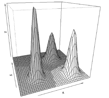
Figure 3. Decision regions for three bivariate normal distributions

Additionally, we consider the case when the element does not belong to any class. To do this, we include a lower limit for the value of the discriminant function, below which the element is not assigned to any class. Figure 4 presents the same example as above, but including a lower limit of 0.10. The code is as follows:

> discriminant.bivariate( mean = mean,
+ sigma = sigma, xlim = c(-3,12),
+ ylim = c(-3,12), col = c(2,7,3),
+ N = 40, threshold = 0.1, theta = -20,
+ phi = 20, ltheta = -120, shade 0.65)
>

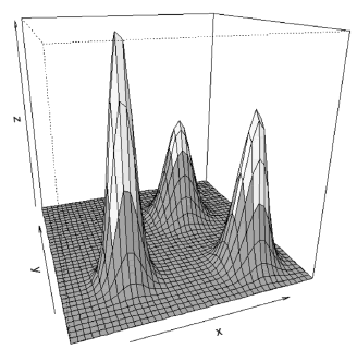
Figure 4. Decision regions for three bivariate normal distributions with a lower limit of 0.010

3.3. Data classification in 2-d
The R language has no direct functions to plot classification plots in 2-D patterns. In this case, we write the classify.2D.plot function with the aim of facilitating the visualization of these problems. The function takes as input an n x 2 matrix representing the coordinates x1 and x2 of n points. Additionally, the parameter d is a binary matrix of n rows by the number of classes in the data; each element of d takes the value 1 when the current pattern belongs to the class, and 0 otherwise.

For the data used in the example above, the call to classify.2D.plot without specifying the classes

> classify.2D.plot(x = cbind(x1, x2))

generates the graph shown in Fig. 5. When we specify a single class, it is assumed that we have a dichotomous classification dataset, and the function generates a graph indicating the specified class for each element in the dataset. The call

> classify.2D.plot(x = cbind(x1, x2),
+ d = cbind(d1+d2))

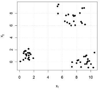
Figure 5. Use of the classify.2D.plot function without specify the classes of the inputs

generates the graph in Fig. 6. When we specify more than one class, each point is displayed with a number indicating to which class it belongs. In Fig. 7, we present the output obtained for

> classify.2D.plot(x = cbind(x1, x2),
+ d = cbind(d1,d2,d3))

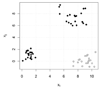
Figure 6. Plot for a classification problem with two classes

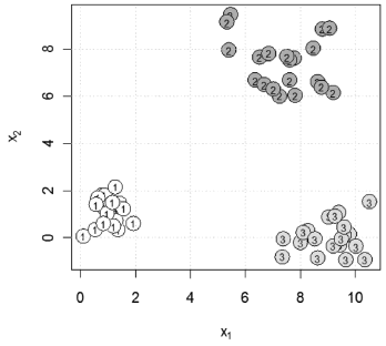
Figure 7. Plot for a classification problem with several classes

In addition, classify.2D.plot is able to receive the parameters of one or more linear classifiers with the aim of plotting the decision boundaries. In Fig. 8, we present the graphic obtained using the following commands:

> classify.2D.plot(x = cbind(x1, x2), d =
+ cbind(d1,d2,d3), intercept = obj$b, coefs = obj$w,
+ density = 20, col = 'gray')

where the coefs and intercept parameters were obtained using the perceptron rule (not illustrated here).

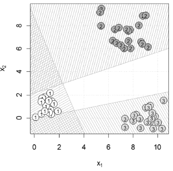
Figure 8. Plot for a classification problem with several classes and decision boundaries

Figure 8, in addition to displaying data and decision boundaries, can illustrate two very important concepts in the field of linear classifiers. Firstly, the empty region in the center of the graph, corresponding to the points not belonging to any class, is easily visualized. Secondly, it is easy to see the regions of points which belong to more than one class; these regions are filled with two or more line patterns.

3.4. Nonlinear decision boundary
Finally, we exemplify how to plot the decision boundary of a nonlinear classifier. The R language has no primitive function that allows the user to plot the contour of a function. In order to meet this need, the contour.2D function was written. The levels parameter is used to specify which contour lines to be plotted are. In order to obtain the contour lines of the decision boundary, it is necessary to set the parameter to an appropriate value depending on the classifier.

The procedure for obtaining the decision boundary will be exemplified for a bipolar XOR function. In this case, the nonlinear classifier is specified as the function g(x1,x2 )=0.667x12-x1 x2+0.667x22-1.333. The decision boundary is obtained for g(x1,x2 )=0. The commands used to obtain Figs. 9 and 10 are the following:

> xor.x = rbind(c(-1, -1), c(-1, +1),
+ c(+1, -1), c(+1, +1))
> xor.d = cbind(c(0, +1, +1 , 0))
> zz <- function(x1, x2) {return (+ 0.667 *
+ x1^2 - 1 * x1 * x2 + 0.667* x2^2 - 1.333)}
> classify.2D.plot(x = xor.x, d = xor.d, xlim
+ = c(-3, 3), ylim = c(-3, 3))
> abline(h = 0, v = 0)
> contour.2D (fn = zz, xlim = c(-3, 3), ylim =
+ c(-3, 3), N = 50, nlevels = 60, levels = 0,
+ col = NULL, add = TRUE, lwd = 2)
>
> surface.3D( fn=zz, xlim=c(-3,3),
+ ylim=c(-3,3), N=40, theta=-25, phi=35,
+ col='gray80', ltheta=-120, shade=0.45 )
>

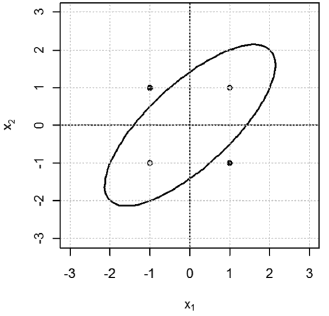
Figure 9. Boundary decision for a nonlinear classifier solving the bipolar XOR problem

 

4. CONCLUSIONS

In this article, we have presented several nontrivial examples of plotting functions in order to illustrate key concepts in the field of pattern classification using the R language. The main objective of this paper is to provide to the reader with practical guidance on building advanced graphics using this computational tool. The work presented is not exhaustive, but it demonstrates the potential of R for the construction of advanced graphics; in addition, it serves as a starting point for the reader to explore other language features, and build their own functions for illustrate problems in the areas of pattern recognition and pattern classification.

 

5. APPENDIX

5.1. The surface.3D function

surface.3D <-
function (fn, fc = NULL, xlim = c(0, 1),
ylim = c(0, 1), N = 20, col = "white", ...)
{
x = seq(xlim[1], xlim[2], length.out = N)
y = seq(ylim[1], ylim[2], length.out = N)
g = expand.grid(x = x, y = y)
z = matrix(fn(g$x, g$y), N, N)
if (!is.null(fc)) {
x.c = x[-N] + 0.5 * (x[2] - x[1])
y.c = y[-N] + 0.5 * (y[2] - y[1])
g = expand.grid(x = x.c, y = y.c)
col = matrix(fc(g$x, g$y), N-1, N-1)
}
persp(x = x, y = y, z = z, col = col, ...)
}

5.2. The discriminant.bivariate function

discriminant.bivariate <-
function (mean, sigma, xlim = c(0, 1),
ylim = c(0, 1), col = "white",
threshold = 0, ...)
{
calc.prob <- function(x, y, flag = 0) {
g = rep(0, times = length(x))
n = rep(1, times = length(x))
for (k in 1:nrow(mean)) {
p = dmvnorm(
x = cbind(x, y),
mean = mean[k, ],
sigma=matrix(sigma[k,],2,2))
n[p > g] = k
g = pmax(p, g)
}
if (flag == 0) {
return(g)
}
else {
if (length(col) == 1)
col = rep(col,
times = nrow(x))
c = col[n]
c[g < threshold] = 8
return(c)
}
}
fn <- function(x, y) calc.prob(x, y, 0)
fc <- function(x, y) calc.prob(x, y, 1)
surface.3D(fn = fn, fc = fc, xlim = xlim,
ylim = ylim, ...)
}

REFERENCES

[1] Jackiw, N., The Geometer's Sketchpad [computer software]. Key Curriculum Press: Emeryville, CA, 2001.         [ Links ]
[2] Jackiw, N. Drawing Worlds: Scripted Exploration Environments in The Geometer's Sketchpad" in "Geometry Turned On!: Dynamic Software in Learning, Visualizing Complex Functions Teaching, and Research", eds. James R. King and Doris Schattschneider (Washington, D.C.: The Mathematical Association of America): 179-184, 1997.         [ Links ]
[3] Laborde, J.M.; Bellemain, F., Cabri Geometry II computer software. LSD2- IMAG Grenoble and Texas Instruments, 1992.         [ Links ]
[4] Wolfram, S., The Mathematica book. Cambridge, UK: Cambridge University Press, 1996.         [ Links ]
[5] Gorjanc, S., Some Examples of Using Mathematica and webMathematica in Teaching Geometry. Journal of Geometry Graphics: 2(8), pp. 243-253, 2004.         [ Links ]
[6] Gorjanc, S., Some Examples of Using Mathematica in Teaching Geometry. Proc. 10th ICGG (International Conference on Geometry and Graphics), Kiev (Ukraine), July 28 - Aug. 3, Vol. 2, pp. 89-93, 2002.         [ Links ]
[7] Balkin, S.D., Taking Calculus with Mathematica. The Mathematica Journal: 4(2), pp. 52-53, 1994.         [ Links ]
[8] Allenby, G.M. and Rossi, P.E. (2008), Teaching Bayesian Statistics to Marketing and Business Students. The American Statistician: 62(3), pp. 195-198, 2008.         [ Links ]
[9] Ihaka, R. and Gentleman, R. (1996), R: A language for data analysis and graphics. Journal of Computational and Graphical Statistics: 5, pp. 299–314, 1996.         [ Links ]
[10] Becker, R., Chambers, J.M. and Wilks, A., The (new) S language: A programming environment for data analysis and graphics. Pacific Grove: Wadsworth & Brooks/Cole, 1998.         [ Links ]
[11] Chambers, J. M., Programming with data: A guide to the S language. New York: Springer-Verlag, 1998.         [ Links ]
[12] Chambers, J.M. and Hastie, T.J., Statistical Models in S. Chapman & Hall, London, 1992.         [ Links ]
[13] Insightful, S-Plus 8 for Windows. User's Guide. Insightful Corporation, Seattle, WA, 2007.         [ Links ]
[14] Fox, J., The R commander: A basic statistics graphical user interface to R. Journal of Statistical Software: 14(9), 2005.         [ Links ]
[15] Sriplung, H., Integrated computing environment for R. R package Version 1.0–1. URL: http://www.r-ice.org., 2006         [ Links ]
[16] Chambers, J. M., Programming with data: A guide to the S language. New York: Springer-Verlag, 1998.         [ Links ]
[17] Chambers, J.M. and Hastie, T. J., Statistical Models in S. Chapman & Hall, London, 1992.         [ Links ]
[18] Grunsky, E.C., R: a data analysis and statistical programming environment -- an emerging tool for the geosciences. Computers Geosciences: 28 (10), pp. 1219-1222, 2002.         [ Links ]
[19] Velásquez, J.D., Olaya, Y. and Franco, C.J., Análisis y predicción de series de tiempo en mercados de energía usando el lenguaje R. DYNA: 78(165), pp. 287-296, 2011.         [ Links ]
[20] Velásquez, J.D., Implementación de una memoria asociativa lineal usando el lenguaje R. Revista Avances en Sistemas e Informática: 7(2), pp. 97-103, 2010.         [ Links ]
[21] Ripley, B.D., Pattern Recognition and Neural Networks. Cambridge University Press, 1996.         [ Links ]
[22] Jang, J.-S.R., Sun, C.-T. and Mizutani, E., Neuro-Fuzzy and Soft Computing: A computational approach to learning and machine intelligence. Prentice Hall, Upper Saddle River, NJ, 1997.         [ Links ]
[23] Duda, R.O., Hart, P.E. and Stork, D.G., Pattern Recognition. John Wiley and Sons. 2001.         [ Links ]