A COMPARISON OF EXPONENTIAL SMOOTHING AND NEURAL NETWORKS IN TIME SERIES PREDICTION

UNA COMPARACIÓN ENTRE EL SUAVIZADO EXPONENCIAL Y LAS REDES NEURONALES EN LA PREDICCIÓN DE SERIES DE TIEMPO

 

JUAN DAVID VELÁSQUEZ HENAO
Profesor Titular, Dpto. de Ciencias de la Computación y de la Decisión, Universidad Nacional de Colombia, jdvelasq@unal.edu.co

CRISTIAN OLMEDO ZAMBRANO PEREZ
Estudiante, Maestría en Ingeniería - Sistemas, Universidad Nacional de Colombia, cozambra@unal.edu.co

CARLOS JAIME FRANCO CARDONA
Profesor Titular, Dpto. de Ciencias de la Computación y de la Decisión, Universidad Nacional de Colombia, cjfranco@unal.edu.co

 

Received for review July 09^th, 2012, accepted August 20^th, 2013, final version October, 15^th, 2013

 

---

ABSTRACT: In this article, we compare the accuracy of the forecasts for the exponential smoothing (ES) approach and the radial basis function neural networks (RBFNN) when three nonlinear time series with trend and seasonal cycle are forecasted. In addition, we consider the recommendations of preprocessing by eliminating the trend and seasonal cycle using simple and seasonal differentiation. Finally, we use forecast combining for determining if there is complementary information between the forecasts of the individual models. Our numerical evidence supports the following conclusions: ES models have a better fit but lower predictive power than the RBFNN; detrending and deseasonality allows the RBFNN to fit and forecast with more accuracy than the RBFNN trained with the original dataset; there is no evidence of information complementarity in the forecasts such that the methodology of forecasts combination is not able to predict with more accuracy than the RBFNN and ES methodologies.

KEYWORDS: Forecasts combination; nonlinear models; artificial neural networks; nonlinear time series.

RESUMEN: En este artículo, se compara la precisión de los pronósticos para la aproximación de suavizado exponencial (ES, por su sigla en inglés) y redes neuronales de función de base radial (RBFNN, por su sigla en inglés) cuando se pronostican tres series no lineales de series de tiempo con tendencia y ciclo estacional. Adicionalmente, se consideran las recomendaciones de preprocesar por medio de la eliminación de la tendencia y del ciclo estacional usando diferenciación simple y diferenciación estacional. Finalmente, se considera el uso de la combinación de pronósticos para determinar si hay información complementaria entre los pronósticos individuales de los modelos. La evidencia numérica soporta las siguientes conclusiones: primero, los modelos de ES tienen un mejor ajuste pero un bajo poder predictivo que las RBFNN; la eliminación del ciclo y la tendencia permite que las RBFNN se ajusten y pronostiquen con mayor precisión que las RBFNN entrenadas con el conjunto original de datos; no hay evidencia de complementariedad de información en los pronósticos, tal que, la metodología de combinación de pronósticos no es capaz de predecir con mayor precisión que las RBFNN y la metodología ES.

PALABRAS CLAVE: combinación de pronósticos; modelos no lineales; redes neuronales artificiales; serie no lineales de tiempo .

---

 

1. INTRODUCTION

The use of methodologies based on statistics, econometrics and artificial intelligence, for the prediction of time series is a popular alternative in financial and energy markets, social sciences and other research areas. This is because forecasts are important inputs in making operational and strategic decisions [1].

In general, forecasting techniques and their applications are very diverse. In [2], a review of the main progress in the last 25 years is done; the authors emphasize the importance gained in the last decade by techniques like exponential smoothing (ES), artificial neural networks and forecast combination, and the importance and relevance of traditional methodologies such as the families of ARIMA and GARCH.

The rise of ES methodologies is because they present a simple structure, which is able to capture the time series components such as the trend and the seasonal cycle. Thus, for example, in [3] and [4] the seasonal component is exploited for forecasting the demands of electricity and natural gas respectively; in [5] and [6], the obtained forecasts are used to control the inventory of car parts.

Artificial neural networks have been received special attention in nonlinear time series forecasting. Typical applications are related with the forecasting of energy consumption [7,8] and electricity prices [9,10]; the difficulty of forecasting is because there are many complex relationships among the market agents [11].

The popularity of forecast combination techniques is explained by the theoretical advances and empirical experiences demonstrating that the combined forecast, usually, is more accurate that the individual forecast of each individual model [12,13]. Current research is mainly focused on obtaining new methods for combining individual forecasts. Thus, for example, forecasts obtained using ES methodology are combined with the forecasts of other alternative models using the Akaike information criterion [14] or novel approaches like the AFTER algorithm [15,16].

Usually, ARIMA and GARCH models are frequently used as benchmarks for comparing the accuracy of diverse models. In [17], GARCH and feed forward artificial neural network models are compared when the stock market indexes of Japan, United Kingdom, Hong Kong and Germany are forecasted. In [8], an ARIMA, a multilayer perceptron neural network (MLP) and an autoregressive neural network are used for forecasting the monthly demand of electricity in the energy Colombian market. In [18], several parametric and semi-parametric models are used for forecasting the electricity prices in California and Norway, are their accuracy is compared.

In time series literature, studies with the aim of comparing the accuracy and determining which are the better techniques in forecasting are common. However, the discussion about this topic remains inconclusive, because there is not a widespread consensus in the scientific community, which accepts the superiority of a specific methodology in relation to another. In contrast, there are many cases reported of the implementation of a limited number of methodologies in a single data set.

With the aim of contributing to the discussion, this paper compares the forecasting ability of exponential smoothing models, neural networks and nonlinear combination of the predictions obtained with the two previous models for three economic series.

The rest of this article is organized as follows. In Section 2, we describe the exponential smoothing, artificial neural networks and forecast combining methodology. Time series datasets are described in Section 3. Next, the obtained results are presented in Section 4. Finally, we conclude in Section 5.

 

2. MATERIALS AND METHODS

2.1. Forecasting methodologies

2.1.1. Exponential smoothing
Exponential smoothing models were developed originally by Holt [19], Brown [20] and Winters [21]. Gardner [24] presents a review of the state of the art and discusses some criteria for model selection. Hyndman et al. [23] incorporate new models and present an equivalent formulation in the form of state space models.

In this article, we use the same nomenclature and the implementation of the exponential smoothing models presented in [22]. Model structure is represented as ES(E, T, S), where E represents the error type [additive (A) or multiplicative (M)], T is the trend [none (N), additive (A), additive damped (AD), multiplicative (M) or multiplicative damped (MD)], and S is the seasonal component [none (N), multiplicative (M) or additive (A)]. Thus, for example, ES(A, N, N) represents a model with additive errors; ES(M, A, M) is a Holt-Winters multiplicative model with multiplicative errors. As discussed by Hyndman et al. [23] there are some methodological and practical restrictions in the use of ES; for example, models with multiplicative errors are not appropriate for datasets with zeros or negative values.

2.1.2. Radial basis function neural network
Artificial neural networks are mathematical models that mimic the physical structure of the brain and their capacity for learning and parallel information processing [26]. Zhang et al. [25] and de Gooijer and Hyndman [2] present reviews about the use of artificial neural networks in time series prediction.

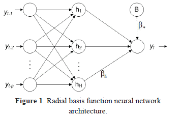
A radial basis function neural network (RBFNN) is a type of feed-forward neural network. The architecture of the RBF neural network is presented in Figure 1; neurons are grouped in three layers: input, hidden and output. The current value of the time series, , is calculated as:

where: is a constant term, are the weights connecting the neurons in the hidden layer to the output; represents the vector of inputs to the RBFNN and corresponds to the previous P values of the time series; H is the number of neurons in the hidden layer; is the activation function of the neurons in the hidden layer, which is defined as:

is a vector of P components and represent the centroid of the neuron h; is the influence radius of the neuron h; and is the Euclidean distance; finally, represents the residual of the model

Model parameters are adjusted in a process of two phases; in the first phase, the parameters and are estimated using a clustering technique or an unsupervised training algorithm; in the second phase, the remaining parameters are calculated using a gradient-based optimization technique.

In this article, we use the notation RBF-I-H for representing the RBFNN with I inputs and H neurons in the hidden layer.

In this study, the number of inputs for a RNFNN is calculated as the optimal order of an autoregressive model fitted to the current dataset, using the Akaike information criterion. For selecting the optimal number of hidden neurons, we use a constructive (additive) approach; first, we fit a model with one hidden neuron; later, with two neurons and so on. The process stops when the fitting error decreases insignificantly. The last fitting model is preferred.

2.1.3. Forecast combining
Forecast combining methodologies are based on the premise that the combination of individual forecasts is more accurate that the forecasts of any individual model [12,13,29,30]. Several alternatives have been proposed for combining individual forecasts, as for example, simple arithmetical average [12], weighted average and several types of nonlinear models [27,28]. However, forecast combining is not useful in all cases and would be better to use an individual forecast [31,32].

In this article, we consider the nonlinear combination of the forecasts of the ES and RBFNN models using a multilayer perceptron neural network. Therefore, the multilayer perceptron has two inputs. As in the case of the RBFNN, the number of hidden neurons is obtained in a constructive way. First, we consider a model with one hidden neuron, later, two hidden neurons and so on.

2.2. Time series datasets

2.2.1. Electricity contract prices
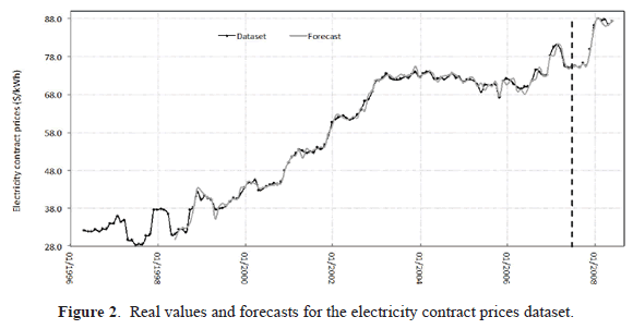
This time series corresponds to the monthly average prices, in $/kWh, of the electricity dispatch in the spot Colombian market for the period from 05/1996 to 06/2008 (146 observations) [35]. This time series is characterized by a local linear trend and a seasonal cycle with an annual period (see Figure 2).

2.2.2. Electricity demand
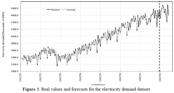
This time series, with 177 observations, corresponds to the monthly demand of electricity for the Colombian energy market, in thousands of GWh, from 08/1995 to 04/2010 [36]. In Figure 3, a plot of this time series is presented.

2.2.3. Paper sales
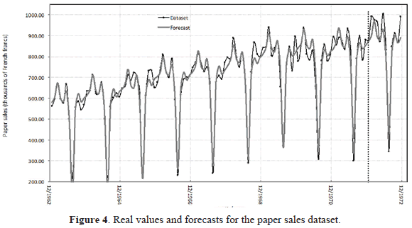
This time series, with 120 observations, contains industry sales for printing and writing paper (in thousands of French francs) from 01/1963 to 12/1972 [37] [38]. The plot of this time series is presented in Figure 4.

2.3. Time series preprocessing
Empirical evidence suggests that multilayer perceptron neural networks are not able to capture the seasonality and the trend present in the time series [33,34]; thus, Nelson et al. [33] and Zhang and Qi [34] recommend the use of the operators of simple and seasonal differentiation for eliminating the trend and the seasonal cycle previous to the fitting of the neural network. However, there is no evidence of this for other types of neural networks. Thus, in this work, we forecast the original time series and the differenced time series with the aim of contributing to the discussion about preprocessing.

2.4. Calculation details
For each time series dataset, we consider two cases:

1. The forecast of the original time series without transformations.
2. The forecast of the transformed time series obtained as where B is the backshift operator . In this case, we eliminate the trend and seasonal cycle by applying the operators of simple and seasonal differentiation (as recommended in [34]).

Each dataset was divided in two samples: the first sample is used for fitting the considered models; the last sample is conformed for the last of 12 observations of the dataset and it is used for forecasting purposes only. In addition, we consider only one-month-ahead forecasts

Forecast accuracy is measured using the mean square error (MSE):

And the mean absolute deviation (MAD):

 

3. RESULTS AND DISCUSSION

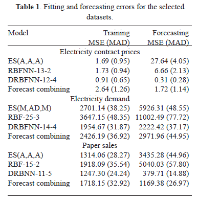
For all datasets, we use the ets() function in the forecast package [22] for fitting and forecasting the ES models. For the ES methodology, we forecast only the original time series (y_t), because this methodology explicitly represents the trend and the seasonal cycle present in the dataset. In Table 1, we report the preferred ES models and the corresponding MSE and MAD for the fitting (training) and forecasting samples.

The RBFNN are fitted to the datasets with and without differentiation as described in Section 2.4. We name the model RBFNN when the neural network is fitted to the original dataset without transformations and DRBFNN for models fitted to the transformed time series. Preferred models were selected as discussed in Section 2.1.2 and the corresponding fitting and forecast errors are presented in Table 1.

Forecast combination is calculated using a multilayer perceptron neural network with two inputs: the first input is the forecast from the preferred ES model; the second input is the forecast from the preferred model between the RBFNN and DRBFNN models. For obtaining the optimal number of hidden neurons, we use a constructive approach as in the case described for the RBFNN in Section 2.1.2.

For each dataset, we plot the best forecast. See Figures 2, 3 and 4.

When the results in Table 1 are analyzed, several conclusions arise:

• ES models present better fitting than RBFNN models. However, ES models are worse in accuracy for out-of-sample forecasts, except in the case of electricity contract prices datasets. Possibly, this is because the contract prices present unusually higher values in the out-of-sample forecast.
• It is better to eliminate the trend and the seasonal cycle when the forecasts are obtained using RBFNN models. For the all datasets, the differentiation allows to the RNFNN to capture subtle dynamics hidden behind the trend and the seasonal pattern; as a consequence, the fitting and forecasting errors for the differenced time series (DRBFNN model) are lower than the obtained for the RNFNN model adjusted to the original dataset; this finding is in concordance with references [33] and [34].
• Forecast combining is not able to generate more accurate forecasts in all datasets. This result indicates that there is not complementary information between the forecasts and, as a consequence, the forecast cannot be improved

 

4. CONCLUSIONS

In this paper, we compare the accuracy of exponential smoothing, radial basis functions neural networks and forecast combining methodology for time series with trend and seasonal cycle. In addition, we evaluate if the accuracy of radial basis function neural network models increases when the trend and the seasonal cycle are eliminated.

The presented evidence indicates: first, that radial basis function neural networks are more accurate than exponential smoothing methods; second, the elimination of trend and seasonal cycle allows the neural network to capture subtle aspects of the dynamics of time series increasing forecast accuracy. And third, forecast combination techniques do not always generate more accurate forecasts than individual models, as enunciated in [31] and [32].

 

BIBLIOGRAPHY

[1] Makridakis, S G., Forecasting: its role and value for planning and strategy. International Journal of Forecasting: 12(4), pp. 513-537, 1996.         [ Links ]
[2] De Gooijer, J.G. and Hyndman, R.J., 25 years of time series forecasting. International Journal of Forecasting: 22(3), pp. 443-473, 2006.         [ Links ]
[3] Taylor, J.W., Short-term electricity demand forecasting using double seasonal exponential smoothing. Journal of the Operational Research Society: 54(8), pp. 799-805, 2003.         [ Links ]
[4] Lee, T.S., Cooper, F.W., and Adam, E.E., The effects of forecasting errors on the total cost of operations. Omega: 21(5), pp. 541-550, 1993.         [ Links ]
[5] Snyder, R.D., Koelher, A.B. and Ord, J.K., Forecasting for inventory control with exponential smoothing. International Journal of Forecasting: 18(1), pp. 5-18, 2002.         [ Links ]
[6] Syntetos, A.A., Boylan, J.E. and Croston, J.D., On the categorization of demand patterns. Journal of the Operational Research Society: 56(5), pp. 495-503, 2005.         [ Links ]
[7] Balestrassi, P.P., Popova, E., Paiva, A.A. and Marangon Lima, J.W., Design of experiments on neural network's training for nonlinear time series forecasting. Neurocomputing: 72(4-6), pp. 1160-1178, 2009.         [ Links ]
[8] Velásquez, J.D., Franco, C.J. and García, H.A., Un modelo no lineal para la predicción de la demanda mensual de electricidad en Colombia. Estudios Gerenciales: 25(112), pp. 37-54, 2009.         [ Links ]
[9] Gareta, R., Romeo, L.M. and Gil, A., Forecasting of electricity prices with neural networks. Energy Conversion and Management: 47(13-14), pp. 1770-1778, 2006.         [ Links ]
[10] Pao, H.-T., Forecasting electricity market pricing using artificial neural networks. Energy Conversion and Management: 48(3), pp. 907-912, 2007.         [ Links ]
[11] Angelus, A., Electricity price forecasting in deregulated markets. Electricity Journal: 4, pp. 32-41, 2001.         [ Links ]
[12] Bates, J.M. and Granger, C.W.J., Combination of forecasts. Operations Research Quarterly: 20(4), pp. 451-468, 1969.         [ Links ]
[13] Clemen, R.T., Combining forecasts: a review and annotated bibliography. International Journal of Forecasting: 5(4), pp. 559-583, 1989.         [ Links ]
[14] Kolass, S., Combining exponential smoothing forecasts using Akaike weights. International Journal of Forecasting: 27(2), pp. 238-251, 2011.         [ Links ]
[15] Zou, H. and Yang, Y., Combining time series models for forecasting. International Journal of Forecasting: 20(1), pp. 69-84, 2004.         [ Links ]
[16] Yang, Y., Combining forecasting procedures: some theoretical results. Econometric Theory: 20(1), pp. 176-222, 2004.         [ Links ]
[17] Hossain, A. and Nasser, M., Comparison of GARCH and neural networks methods in financial time series prediction. Proceedings of 11th International Conference on Computer and Information Technology (ICCIT 2008), pp. 729-744, 2008.         [ Links ]
[18] Weron, S. and Misiorek, A., Forecasting spot electricity prices: A comparison of parametric and semiparametric time series models. International Journal of Forecasting: 24(4), pp. 744-763, 2008.         [ Links ]
[19] Holt, C.C., Forecasting seasonals and trends by exponential weighted moving averages, ONR Research Memorandum, vol. 52, Available from the Engineering Library, University of Texas at Austin, 1957.         [ Links ]
[20] Brown, R.G., Statistical forecasting for inventory control. New York: McGraw-Hill, 1959.         [ Links ]
[21] Winters, P.R., Forecasting sales by exponentially weighted moving averages. Management Science: 6(3), pp. 324-342, 1960.         [ Links ]
[22] Hyndman, R.J. and Khandakar, Y., Automating time series forecasting: the forecast package for R. Journal of Statistical Software: 27(3), 2008. Recupered from http://www.jstatsof.org.         [ Links ]
[23] Hyndman, R.J., Koehler, A.B., Snyder, R.D. and Grose, S., A state space framework for automatic forecasting using exponential smoothing methods. International Journal of Forecasting: 18(3), pp. 439-454, 2002.         [ Links ]
[24] Gardner, E.S., Exponential smoothing: The state of art, Part II. International Journal of Forecasting: 22(4), pp. 637-666, 2006.         [ Links ]
[25] Zhang, G., Patuwo, B., and Hu, M., Forecasting with artificial neural networks: the state of art. International Journal of Forecasting: 14(1), pp. 35-62, 1998.         [ Links ]
[26] Masters, T., Practical Neural Networks Recipes in C++. New York: Academic Press, 1993.         [ Links ]
[27] Fiordaliso, A., A nonlinear forecasts combination method based on Takagi-Sugeno fuzzy systems. International Journal of Forecasting: 14(3), pp. 367-379, 1998.         [ Links ]
[28] Terui, N. and van Dijk, H.K., Combined forecasts from linear and nonlinear time series models. International Journal of Forecasting: 18(3), pp. 421-438, 2002.         [ Links ]
[29] Armstrong, S., Combining forecasts: the end of the beginning or the beginning of the end?. International Journal of Forecasting: 5(4), pp. 585-588, 1989.         [ Links ]
[30] Makridakis, S., Andersen, A., Carbone, R., Fildes, R., Hibon, M., Lewandowski, R., Newton, J., Parzen, E. and Winkler, R., The accuracy of extrapolation (time series methods): results of a forecasting competition. Journal of Forecasting: 1(2), pp. 111-153, 1982.         [ Links ]
[31] Larrick, R. and Soll, J., Intuitions about combining opinions: misappreciation of the averaging principle. Working paper INSEAD, 2003/09/TM.         [ Links ]
[32] Hibon, M. and Evgeniou, T., To combine or not to combine: selecting among forecasts and their combinations. International Journal of Forecasting: 21(1), pp. 15-24, 2005.         [ Links ]
[33] Nelson, M., Hill., T., Remus, T. and O'Connor, M., Time series forecasting using neural networks: Should the data deseasonalized first?. Journal of Forecasting: 18(5), pp. 359-367, 1999.         [ Links ]
[34] Zhang, G. and Qi, M., Neural networks forecasting for seasonal and trend time series. European Journal of Operational Research: 160(2), pp. 501-514, 2005.         [ Links ]
[35] Velásquez, J.D. and Franco, C.J., Predicción de los precios de contratos de electricidad usando una red neuronal con arquitectura dinámica. Innovar Journal: 20(36), pp. 7-14, 2010.         [ Links ]
[36] Franco, C.J., Velásquez, J.D. and Olaya, Y., Caracterización de la demanda mensual de electricidad en Colombia usando un modelo de componentes no observables. Cuadernos de Administración: 21(36), pp. 221-235, 2008.         [ Links ]
[37] Makridakis, S.G., Wheelwright, S.C. and Hyndman, R.J., Forecasting: Methods and applications. New York: John Wiley & Sons, 1998.         [ Links ]
[38] Ghiassi, M., Saidane, H. and Zimbra, D.K., A dynamic artificial neural networks for forecasting time series events. International Journal of Forecasting: 21(2), pp. 341-362, 2005.         [ Links ]