http://dx.doi.org/10.15446/dyna.v81n183.34745

SIMULTANEOUS LOCALIZATION OF A MONOCULAR CAMERA AND MAPPING OF THE ENVIRONMENT IN REAL TIME

LOCALIZACIÓN DE UNA CÁMARA MONOCULAR Y MAPEO SIMULTÁNEO DEL ENTORNO EN TIEMPO REAL

 

ANDRÉS DÍAZ
Magister , Grupo de Percepción y Sistemas Inteligentes, Universidad del Valle-Cali, andres.a.diaz@correounivalle.edu.co

LINA PAZ
Dra en Sistemas e Informática, Grupo de Robótica, Percepción y Tiempo Real, Universidad de Zaragoza, linapaz@unizar.es

EDUARDO CAICEDO
Dr en Informática, Grupo de Percepción y Sistemas Inteligentes, Universidad del Valle-Cali, eduardo.caicedo@correounivalle.edu.co

PEDRO PINIÉSS
Dr en Ingeniería de Sistemas, Grupo de Robótica, Percepción y Tiempo Real, Universidad de Zaragoza, ppinies@unizar.es

 

Received for review November 03^th, 2012, accepted October 18^th, 2013, final version december, 12^th, 2013

 

---

ABSTRACT: In this work a Visual SLAM system (Simultaneous Localization and Mapping) that performs in real time, building feature-based maps and estimating the camera trajectory is presented. The camera is carried by a person that moves it smoothly with six degrees of freedom in indoor environments. The features correspond to high quality corners parametrized with inverse depth representation. They are detected inside regions of interest and an occupancy criterion is applied in order to avoid feature agglomeration. The association process is developed using active search. The final representation is made in a three-dimensional environment.

Keywords: Localization, mapping, EKF, monocular camera, inverse depth, real time, 6DOF, active search.

RESUMEN: En este trabajo se presenta el desarrollo de un sistema de SLAM Visual (Simultaneous Localization and Mapping) que se desempeña en tiempo real, construyendo mapas basados en puntos característicos y estimando la trayectoria de la cámara. La cámara es transportada por una persona que la mueve suavemente con seis grados de libertad en entornos interiores. Los puntos característicos corresponden a esquinas de alta calidad parametrizados con el inverso de su profundidad. Estos son detectados dentro de regiones de interés y se aplica un criterio de ocupación con el fin de evitar aglomeración de características. El proceso de asociación se desarrolla usando búsqueda activa. La representación final se realiza en un entorno tridimensional.

Palabras Clave: Localización, mapeo, EKF, cámara monocular, inverso de la profundidad, tiempo real, 6DOF, búsqueda activa.

---

 

1. INTRODUCTION

Before carrying out tasks such as navigation, path planning, and object and place recognition, a totally autonomous mobile robot must interpret the information obtained by its sensors and then estimate its position and the position of environmental features. The simultaneous localization and map building algorithms face both problems at the same time [1], and they have been the focus of attention of the research community on mobile robotics during the last two decades.

The system described in this article is able to estimate the camera position, which is carried by a person or by a mobile platform, and to represent the trajectory that it makes. The system creates a three-dimensional map composed of the camera model and spatial points that represent object corners in the environment. Moreover, it can be adapted to different mobile platforms -terrestrial, aquatic, and aerial- because it is portable and has six degrees of freedom that reduce motion restrictions. The system is of great importance when GPS information is not available and in applications where is not practical to carry heavy and bulky sensors such as object tracking and mapping of environments in rescue operations.

Section 2 defines the schema of the Visual SLAM system and the general methodology used in this work. Section 3 presents outstanding projects about Visual SLAM. Sections 4 and 5 explain how the key points were detected and how the radial distortion was corrected, respectively. Sections 6, 7, 8 and 9 present the parametrization process with the inverse depth of the features, the constant velocity model, the prediction of feature location in the image plane and the data association, respectively. Finally, the results and conclusions obtained in this work are presented.

 

2. VISUAL SLAM

Recently, the use of visual sensors has generated great interest in the research field of SLAM due to the large amount of texture information provided by these sensors of the objects found in a scene [2-4]. Moreover, cameras are compact, accurate, and much cheaper than laser sensors.

Implementations such as the ones developed by Castellanos [5] and Davison [6] proved the EKF (Extended Kalman Filter) in the building of small maps in SLAM systems with stereo vision, working in real time at 5 Hz. The system was able to build three-dimensional maps and to control a mobile robot. Jung and Lacroix [7] developed an autonomous system for mapping terrains using stereo vision as the only sensor and the standard EKF. Saez [8] presented a SLAM system with stereo vision for six degrees of freedom movements and indoor environments.

Some SLAM systems that use a monocular camera have proved to be viable in small environments; the most outstanding systems are the ones designed by Bailey [9], Kwok [10] and Lemaire [11]. Most of them are essentially EKF-SLAM systems and only change the initialization techniques and the kind of interest points extracted from the images (Harris corners, Shi and Tomasi corners, SIFT features, or any mixture of them). The works of Civera [12], Tully [13], Clemente [14] and Marzorati [15] show a tendency to use monocular cameras, inverse depth parametrization, and to perform in real time. The sub-mapping techniques, such as the ones depevoped by Bosse [16], Leonard [17], Paz [18] and Piniés [19], allow the system to achieve a performance in long trajectories.

 

3. SCHEMA OF OUR SLAM SYSTEM

The SLAM system involves many processes that work together in sequential way as is shown in Fig. 1. The probabilistic core is the EKF that alternates between a prediction step and an update step. Every process has inputs and outputs that are in a chain that ends up in a state estimate. In the next sections, these variables and their functions in the whole process are explained.

 

4. CORNER DETECTION

The system begins getting information of the environment through key points; in this work the corners are obtained with the Harris detector, supported by OpenCV. The image is split in 36 region of interest and for each region the Harris detector is applied, returning the best corner. From them, the corners with their minimum eigenvalue over a given threshold are chosen and only five of them are initialized, the best corners. At the beginning all the regions are empty, but after the first iteration, an occupancy algorithm must be used in order to avoid agglomeration of corners and therefore, wrong associations. In this step the coordinates of the five best corners are stored, the regions where they were found and a patch of 15x15 pixels around each corner.

4.1. Occupancy Algorithm
This criterion defines empty and occupied regions of interest. Only empty regions can be used to initialize a new feature. Moreover, when a region becomes empty because both the feature was deleted or the feature moves to another region, 20 time steps must pass in order to consider this region available to be occupied again. This technique allows the features to be well distributed over the image plane.

 

5. CORRECTION OF RADIAL DISTORTION

The corner coordinates have radial distortion that affects the location of the pixels and this displacement grows as the pixel nears the image boundary. The model that describes this distortion is shown in (1).

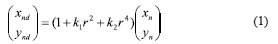
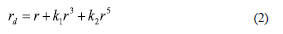
where k1 and k2 are the coefficients of radial distortion, r is the radius, xn and yn are the normalized coordinates. This model allows the system to include radial distortion. However, the opposite process is needed (remove radial distortion) and there is no analytical function that does this. Therefore, a numerical method is employed, the Newton Raphson method, that use the expression (2) and its derivative in order to calculate an approximation of the radius without distortion.

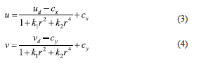
Given the radius r, the principal point (Cx,Cy) and the image coordinates with distortion (ud,vd), the image coordinates without distortion (u, v) can be computed using the expressions (3) and (4). Hereafter the corners will be called features.

 

6. FEATURE INITIALIZATION

This step consists in the corner parametrization and its inclusion to the state vector. The explanation of the corner parametrization using inverse depth representation and the addition of features in the state vector will be presented in this section.

6.1. Inverse Depth Representation
A significant limitation of the initial approaches of Davison [2] and others was that the systems could only use features close to the camera and that had great parallax during the motion. This problem limited the robot navigation (or the camera navigation) to indoors. Montiel [20] proposed a technique to initialize features using the inverse distance between the feature and the camera where it was seen for first time. This technique allows the system to work with both close and distant features from the moment they are detected. The distant features are used to improve the motion estimation, acting initially as an orientation reference. These features are common in outdoor environments.

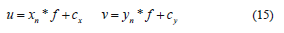
The coordinates (u, v) are used in the back projection model, obtaining normalized coordinates xn and yn:

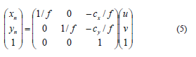
where f is the focal length and (cx,cy) is the principal point. The normalized coordinates give information about the ray hc that passes through the optical center of the camera and the point in the world whose image coordinates are (ud, vd). The ray can be defined by the angles ? and F, the azimuth and the elevation angles respectively:

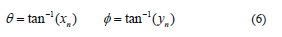
The camera state is defined with six parameters:

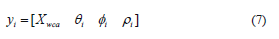
The vector Xwca = [xwc ywc zwc]T corresponds to the camera location, in Cartesian coordinates, from where the features were seen for first time, ?i is the azimuth angle, fi is the elevation angle and ?i = 1/di is the inverse distance between the camera position and the feature.

6.2. Addition of Features to the State Vector
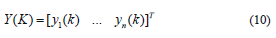
The state vector stores the information of the camera and outstanding features:

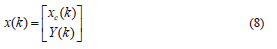
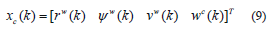
where rw corresponds to the three cartesian coordinates of the camera location, ?w is the camera orientation in Roll, Pitch, Yaw angles [?x, ψy, ψz]T , vw is the linear velocity of the camera and ?c is the angular velocity with respect to the camera frame. The vector Y (k) contains the information of the environment, organized by set of features taken from different camera locations:

where each feature yi was defined in equation (7). A feature initialized remains in the state vector for the whole execution if this overcomes the following criterion: the feature must be seen at least 17 times in the first 20 iterations, from the time it was detected. If certain feature overcomes this criterion, it will not be deleted from the state vector and will be predicted in every iteration.

 

7. MOTION MODEL

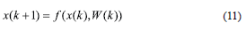
The camera is connected to a laptop and is carried by a mobile robot or by a person. A program on the laptop determines the trajectory and builds a map with well distributed features in real time. The camera moves freely in three dimensions in an unknown environment. A constant linear and angular velocity model is used. The motion model allows the system to estimate the state transition in order to predict the camera position in the next time step before getting a new observation of the environment. The motion model is a non-linear function that only affects the camera state because the features are assumed to be static. The following transition function is used to pass from the state xk to the state xk+1:

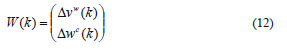
The vector W(k) represents a zero-mean Gaussian noise with covariance Q that affects the linear and angular velocities of the camera to detect small changes in the model:

The camera state xc evolves according to the following expression:

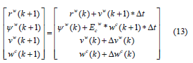
Where Ecw is a matrix that transforms angular velocities with respect to the camera frame to equivalent angular velocities in the world frame.

 

8. PREDICTION OF THE FEATURE LOCATION

This process consists in predicting the feature location in the next image, without making a new observation. Figure 2 provides a graphical representation of the vectors of the camera and feature location.

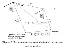
The vector tfvi represents the camera location from where a feature i was observed for first time. The vector defined by m, the unitary vector of the bearing of the feature i when this feature was seen for the first time, this represents the feature location with respect to the vector tfvi. The sum of these vectors is equal to vector featiw, the feature location with respect to the world frame.

The vector tw represents the current camera position, estimated with the motion model described in section 7. The difference of tw and featiw is equal to the vector hw. This vector has to be transformed to the camera frame, obtaining hc. The equation used to predict the azimuth and elevation angles of a feature is based on the components of the vector hc, [hcx, hcy, hcz]:

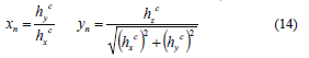
The coordinates (u, v) are calculated from the normalized coordinates xn and yn:

 

9. DATA ASSOCIATION

The location in the image plane (ui, vi) where the features feati will be observed, for i = 1, 2, 3, ..., n, is predicted together with the innovation covariance matrix Si. This matrix defines an elliptical zone of uncertainty where there is high probability to re-observe the feature. In this zone a correlation algorithm is executed, comparing the distribution of the digital levels of the pixels. The location that shows the strongest similarity will be taken as the equivalent point to the central pixel of a corner patch and will be the observed position of the feature from the new camera position.

In Fig. 3 the predictions of feature locations (red points) into the image plane are shown. The blue ellipses indicate failed correlations and therefore, there is no new observation. The green ellipses indicate successful correlations and the new observation is drawn in blue. The yellow point corresponds to a new observation that was parametrized and included into the state vector. This new feature is over an empty and available region and its distance to any other feature is more than 30 pixels.

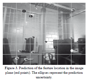
A joint compatibility test based on the Mahalanobis distance is carried out to deal with spurious associations between observations and predicted features that come from dynamic objects in the mapped environment.

When the uncertainty of a feature increases so much, the search zone is too big and it is not suitable to develop the correlation process. In this case this prediction is not used, but the feature is not deleted, it remains in the state vector.

Finally, the difference between the observed feature (blue point) and predicted feature (red point) is the innovation vector and it is used by the Extended Kalman Filter to update the joint state camera-features. This vector moves the estimated position in the direction in which it is reduced.

 

10. RESULTS

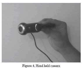
The experiments were developed with the Logitech Pro 9000 camera connected to a HP laptop with a 2.2 GHz AMD Dual-core processor. The camera was carried by a person (Fig. 4) that moves it smoothly with six degrees of freedom, in unknown environments.

10.1. Open Trajectory in Indoor environments

The first experiment was performed in the Laboratory of the Perception and Smart Systems Group. It is a small room with glass walls, chairs, and desks with monitors, printers, CPUs, among other things (Fig. 5). Some corners over the walls belong to reflections and produce failed correlations (blue ellipses in Fig. 3) so most of them are rejected by the high quality features criterion.

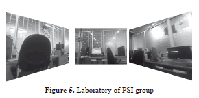
Figure 6 show the corners (points), the camera (triangular prism) and its trajectory (points connected by segments), represented in a three dimensional environment, developed with OpenGL.

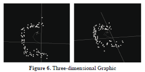
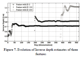
Figure 7 shows how the inverse depth estimates evolve over time. The inverse depth of a feature is initialized with a predefined value with respect to the camera location when the feature is seen for first time. The camera is both rotated and translated and the inverse depth estimate converges to a given value after about 50 iterations. At steady state, the estimates do not vary significantly, which means that the map is consistent. Finally, these estimates are used to compute the feature locations with respect to a global frame.

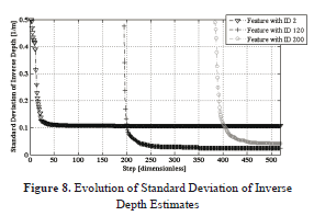
As time passes, the parallax angles increase, yielding better estimates of the inverse depth, which is evidenced by a reduction in standard deviation, as can be seen in Fig. 8.

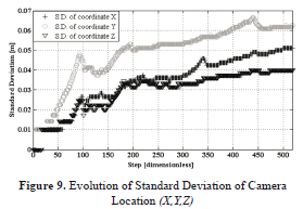
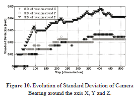
As the camera moves, its own pose uncertainty increases (Figs. 9 and 10). This fact is due to the errors introduced by the motion and observation models and the linear approximations made by the EKF. However, something very interesting happens when a loop is closed. This fact will be seen in the following experiment.

10.2. Closed Loop in Indoor Environments

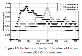
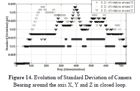
This experiment was carried out with the camera focusing objects over a desk (Fig. 11), trying to follow a square trajectory and to keep a constant distance from the camera to the surface of the desk. The scale of the trajectory was fixed by hand because it is not observable with a monocular camera.

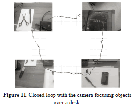
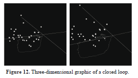
Figure 12 shows the square trajectory and the corners represented with OpenGL.

The camera observes features that were seen in the beginning of the mapping and whose location is relatively well known. Through these observations the uncertainty in camera position (location and orientation) is reduced as is shown in Figs. 13 and 14. These observations also reduce the uncertainty for other features in the map due to the correlation stated in the covariance matrix.

 

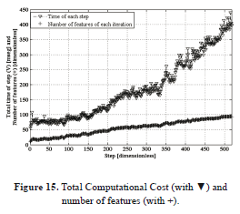
10.3. Computational Cost
The high computational cost is the main limitation in systems that perform in real time. This problem has been tackled with sub-mapping techniques that allow the system to navigate in large environments and to reduce the errors due to the linear approximations made by the Extended Kalman Filter.

Figure 15 depicts the quadratic dependence on the number of features in the map. This fact is due to the size of the covariance matrix that is used to update the state. The matrix operations that involve the covariance matrix are computationally expensive and impose a limit of the number of features to 50 in order to perform in real time, managing to process at least 10 images per second (at the critical point).

 

11. CONCLUSIONS

A Visual SLAM system that works with a monocular camera in real time was developed. The core of the system relies on the well known incremental Extended Kalman Filter such that the positions of camera and a feature-based map can be estimated in real time. The kind of sensor, the 6 DOF and the probabilistic focus used to solve the problem, make it a complex system. The results show that the system performs in indoor environments in real time if the amount of features is under 50, processing from 10 to 20 frames per second.

The estimated state of the camera has low uncertainty: the standard deviation in location is less than 7cm (for each coordinate) and in orientation is less than 3 degrees (for each axis). The inverse depth estimates of landmarks converge to a steady state in about 50 iterations, building consistent maps.

The feature detection is performed using regions of interest and an occupancy algorithm is implemented to avoid feature agglomeration, achieving high quality corners that are well distributed. The elliptical zones defined by the innovation covariance matrix allow the system to carry out an active search of corner patches, optimizing the correlation process. However, the matrix operations increase the computational cost and set a limit to real time performance.

An interesting fact was analyzed, with closed loops the uncertainty decreases when the camera visits a place where it has been before, and recognizes features that were seen before.

 

REFERENCES

[1] Smith, R. C., and Cheeseman P. On the representation and estimation of spatial uncertainty. Int. J. Robotics Research, 5(4): pp.56-68, 1986.         [ Links ]

[2] Davison, A. J., and Murray, D. W. Simultaneous localization and map-building using active vision. IEEE Trans. Pattern Analysis and Machine Intelligence, 24(7): pp.865-880, 2002.         [ Links ]

[3] Davison, A. J., Reid, I. D., Molton, N. D., and Stasse, O. Monoslam: Real-time single camera slam. IEEE Trans. Pattern Analysis and Machine Intelligence, 29(6):pp.1052-1067, June 2007.         [ Links ]

[4] Quintián, H., Calvo, J. L., and Fontenla, O. Aplicación de un robot comercial de bajo coste en tareas de seguimiento de objetos. Revista Dyna, 175, pp.24-33, 2012.         [ Links ]

[5] Castellanos, J. A. Mobile Robot Localization and Map Building: A Multisensor Fusion Approach. PhD thesis, Dpto. de Informática e Ingeniería de Sistemas, University of Zaragoza, Spain, May 1998.         [ Links ]

[6] Davison, A.J. Mobile Robot Navigation using Active Vision. PhD thesis, University of Oxford, 1998.         [ Links ]

[7] Lacroix, S., and Jung, I. K. High resolution terrain mapping using low altitude aerial stereo imagery. In Proc. of the 9th Int. Conf. on Computer Vision, pages pp.946-951, 2003.         [ Links ]

[8] Saez, J.M., Escolano, F., and Penalver, A. First Steps towards Stereobased 6DOF SLAM for the Visually Impaired. In Proc. IEEE Computer Society Conf. on Computer Vision and Pattern Recognition (CVPR'05)- Workshops-Volume 03. IEEE Computer Society Washington, DC, USA, 2005.         [ Links ]

[9] Bailey, T. Constrained initialization for bearing-only SLAM. In Proc. IEEE Int. Conf. on Robotics and Automation, (ICRA'03), volume 2, 2003.         [ Links ]

[10] Kwok, N. M., Dissanayake, G. An efficient multiple hypothesis filter for bearing-only SLAM. In Proc. IEEE/RSJ Int. Conf. on Intelligent Robots and Systems, (IROS'04)., volume 1, 2004.         [ Links ]

[11] Lemaire, T., Lacroix, S., and Sola, J. A practical 3D bearing-only SLAM algorithm. In Proc. IEEE/RSJ International Conference on Intelligent Robots and Systems, (IROS'05), pp. 2449-2454, 2005.         [ Links ]

[12] Civera, J., Davison, A. J., and Montiel, J. M. Inverse depth parametrization for monocular SLAM. IEEE Transactions on Robotics, 24(5): pp932-945, October 2008.         [ Links ]

[13] Tully, S., Moon, H., Kantor, G., and Choset, H. Iterated filters for bearing-only slam. In IEEE International Conference on Robotics and Automation, 2008.         [ Links ]

[14] Clemente, L., Davison, A. J., Reid, I. D., Neira, J., and Tardos, J. D. Mapping large loops with a single hand-held camera. In Proc. Robotics: Science and Systems, Atlanta, GA, USA, June 2007.         [ Links ]

[15] Marzorati, D., Matteucci, M., Migliore, D., and Sorrenti, D. On the use of inverse scaling in monocular slam. In IEEE International Conference on Robotics and Automation, 2009.         [ Links ]

[16] Bosse, M., Newman, P. M., Leonard, J. J., Soika, M., Feiten, W., and Teller, S. An atlas framework for scalable mapping. In Proc. IEEE Int. Conf. Robotics and Automation, pp. 1899-1906, Taipei, Taiwan, 2003.         [ Links ]

[17] Leonard, J. J., and Newman, P. M. Consistent, convergent and constant time SLAM. In Int. Joint Conf. Artificial Intelligence, Acapulco, Mexico, August 2003.         [ Links ]

[18] Paz, L. M., Tardós, J. D., Neira, J. Divide and Conquer: EKF SLAM in O(n). Accepted in Transactions on Robotics (in Print), 24(5), October 2008.         [ Links ]

[19] Piniés, P., and Tardós, J. D. Large Scale SLAM Building Conditionally Independent Local Maps: Application to Monocular Vision. Accepted in Transactions on Robotics (in print)., 24(5), October 2008.         [ Links ]

[20] Montiel, J. M., and Civera, J., Davison, A. J. Unified inverse depth parametrization for monocular SLAM. In Proc. Robotics: Science and Systems, Philadelphia, USA, August 2006.         [ Links ]