


Services on Demand
Journal
Article
 English (pdf)
 Article in xml format
 Article references
 Send this article by e-mail
Indicators
-
 Cited by SciELO
 -
 Access statistics
Related links
-
 Cited by Google
 -
 Similars in
SciELO
Similars in
SciELO -
 Similars in Google
Share

 Permalink
DYNA
Print version ISSN 0012-7353
Dyna rev.fac.nac.minas vol.81 no.186 Medellín July/Aug. 2014
https://doi.org/10.15446/dyna.v81n186.40388
http://dx.doi.org/10.15446/dyna.v81n186.40388
Numerical and experimental preliminary study of temperature distribution in an electric resistance tube furnace for hot compression tests
Estudio preliminar numérico y experimental de la distribución de temperatura en un horno tubular de resistencia eléctrica para ensayos de compresión en caliente
Gabriel Torrente-Prato a & Mary Torres-Rodríguez b
a Departamento de Mecánica, Universidad Simón Bolívar, Venezuela, gtorrente@usb.ve
b Departamento de Mecánica, Universidad Simón Bolívar, Venezuela, matorres@usb.ve
Received: October 19th, de 2013. Received in revised form: January 24th, 2014. Accepted: February 25th, 2014
Abstract
Hot compression tests are performed when jaws, each one with a jacketed section to cool a part of its length, move through a tube furnace at elevated temperatures to compress a metal sample between them, changing the boundary conditions and the temperature distribution inside the furnace during the test. This paper presents a preliminary study about the variation of temperature inside a furnace for hot compression tests, when the jaws are positioned inside it. It also proposes a theoretical simulation to determine the temperature profile in the furnace, which is compared with experimental measurements. Both experimental measurement and simulation showed that the temperature inside the tube furnace for hot compression tests is not uniform. By comparing the simulated values with experimental measurements, it can be concluded that the simulation proposed in this paper is a useful tool which estimates the temperature inside a tube furnace in hot compression tests with an acceptable approximation (error less than 4.73%).
Keywords: hot compression tests, electric resistance tube furnaces, temperature distribution, heat balance, convection, radiation.
Resumen
Los ensayos de compresión en caliente se realizan cuando mordazas, refrigeradas en una parte de su longitud, avanzan a través del interior de un horno tubular a temperatura elevada para comprimir una muestra metálica dentro de ellas, ocasionando que las condiciones de frontera y la distribución de temperatura dentro del horno cambien durante el ensayo. Este trabajo presenta un estudio preliminar acerca de la variación de temperatura en el interior de un horno para ensayos de compresión en caliente a medida que las mordazas se posicionan en su interior. Se propone una simulación para determinar teóricamente el perfil de temperatura en el horno, el cual se compara con mediciones experimentales. Los valores experimentales y simulados mostraron que la temperatura dentro del horno para ensayos de compresión en caliente no es uniforme, con una aproximación aceptable (error menor del 4,73%). Se concluye que la simulación propuesta en este trabajo representa una herramienta útil para estimar la temperatura dentro del horno en los ensayos de compresión en caliente.
Palabras clave: ensayos de compresión en caliente, horno tubular de resistencia eléctrica, distribución de temperatura, balance de calor, convección, radiación.
1. Introduction
Most industrial hot forming processes are developing during the cooling of the material being worked. It is not possible to completely insulate the working material, therefore the forming cannot be performed under adiabatic conditions [1, 2].
Extensive studies of hot forming processes, like rolling, wire drawing, and extrusion show that the temperature is one of the process variables that most affect the mechanical behavior of metals and alloys [3, 4].
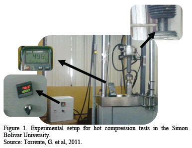
Hot compression tests can better describe the mechanical behavior of metals and alloys during hot forming operations [4]. This has increased the interest in the study of these tests, for example, those made by Kolmogorov [5] in 1937 and Lutton and Sellar [6] in 1969, and more recently those by Cabrera et al. [7] in 1997, Garcia et al. [8] in 2001, Omar et al. [9] in 2006 and Torrente et al. [2] in 2011. As a result of their studies, they all agree that temperature plays an important role in the mechanical behavior of hot formed materials; therefore, it is of interest to understand the thermal behavior inside furnaces used in hot compression tests. This test involves compressing a sample or metallic specimen between the flat faces of two jaws subjected to a test press. During compression, both the specimen and the uncooled portion of the length the jaws, are inside of tube furnace. To perform the test at high temperatures, the furnace is turned so that the sample reaches the desired temperature, but there are discrepancies between the furnace temperature and that of the specimen, making it difficult to establish a value for the temperature when evaluating the behavior of the compressed metal. Therefore, it is important to use numerical simulation to establish and to predict the variation of the temperature inside the furnace, particularly in the region between the jaws. Fig. 1 shows the experimental setup for hot compression tests in the mechanical properties laboratory of the Simon Bolivar University [2,10].
The study of the temperature profiles inside furnaces has been of interest since they began to be used in the Roman era, but only recently, with the popularization of computers, it has been possible to simulate numerically these profiles. Thesis and articles have developed several numerical simulations to clarify thermal profiles in different furnaces, such as the studies presented by Zhaoa et al. [11], Paulsen et al. [12], Ahanj et al. [13], Cawley et al. [14], and Obregon et al. [15] and the theses of Gomez [16], Lee [17] and Courtin [18]. These works developed numerical and experimental studies on different types of natural convection furnaces used for various applications, none of them used for compression tests. The main difference is that in the present work, refrigerated jaws enter the furnace, modifying the temperature profile inside it. This paper presents a preliminary numerical analysis which aims to study the effect of the distance between the jaws in the temperature distribution inside an electric resistance tube furnace for compression tests. The results are compared with some experimental measurements to validate their approach.
2. Experimental measurements
Equipment for performing hot compression tests is shown in Fig. 1 and the experimental setup to measure the temperature, at different points in the furnace for hot compression tests, is shown in Fig. 2.
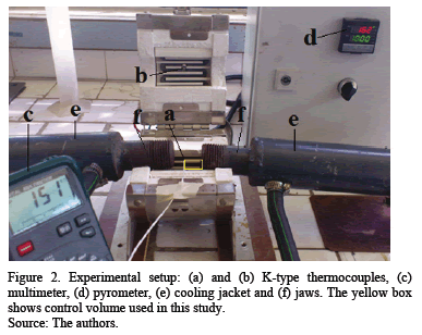
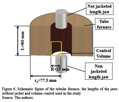
The experimental setup in Fig. 2 shows an electric resistance furnace ATS ® 2961, with a cylindrical body of 25 mm internal radius (R) and 80 mm length (L), whose temperature profile is desired to be established in this work. Also, it shows a detail of the opened furnace and the jaws inside it; these last are solid cylinders of steel AISI H-30 of
15 mm radius and 200 mm length and are used in order to compress metallic samples. These jaws are cooled in order to maintain the temperature in the load cell within its operating range. Therefore, each jaw has a jacketed section of 150 mm length refrigerated with ethylene glycol (Fig. 2-e) and a non-jacketed section of 50 mm length (Fig. 2-f); the last section has a radius of 15 mm which can be introduced inside the furnace.
Experimental temperature measurements were carried out at two points inside the furnace: in the center of the furnace (Fig. 2-a) and on furnace wall (Fig. 2-b) with a type K Thermocouple, recording the temperature of the furnace center with a multimeter MASTECH ® MAS-345 (Fig. 2-c), and on the furnace wall with a pyrometer TAIE ® FY400 (Fig. 2-d).
The Saws areare centered inside the furnace in order to perform the temperature measurements (Fig. 2-f) with specific separations between them of 80, 60, 40, 20 and 0 mm. Once centered, the furnace is closed and the temperature is set to 1273 K. Then the registration of temperatures is carried out with the multimeter and the pyrometer (Figs. 2-a and 2-d, respectively) for the necessary time until they stabilize at a value. The ambient temperature and that registered at the beginning of the test were both 298 K. Forty measurements were recorded of the temperature in the center and on the furnace wall, for each distance between the jaws, performing each experiment in triplicate.
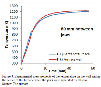
The graphs in Figs. 3 to 5 illustrate some of the curves obtained from experimental temperature measurements made in the center and on the furnace wall when the jaws were separated from each other a distance of 80 mm, 40 mm and 20 mm, respectively. In all of them it is observed a similar behavior, with a rapid rise in temperature to reach the steady state.
Fig. 3 shows the results of the tests when the jaws were 80 mm apart. This figure shows the temperature values in the center and on the furnace wall are similar during heating, the temperature on the furnace wall was only 15 degrees higher.
Figs. 4 and 5, show that the difference in temperature between the center and the furnace wall increases and that this difference increases as the jaws move closer. For the curves in Fig. 4, the temperature of the furnace wall is 58 K higher than the temperature in the center, while for Fig. 5 this difference increases to 118 K.
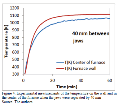
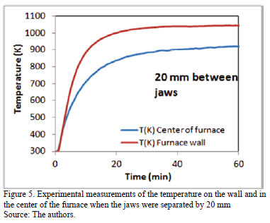
All of the experimental measurements (Figs. 3, 4 and 5) show that at the beginning of the test, the temperature in the center of the furnace is slightly higher than that of the wall. Later on, the temperature on the wall is higher than in the center, and this remains so, even in steady state. This interesting unsteady behavior was not studied numerically, but is worth noticing that it is possibly due to heat transfer to the still cold wall of the furnace being greater than the heat transfer toward the center of the furnace.
3. Governing equations
The finite difference method is used to perform the simulation of the temperature profile, using equations of heat transfer. The simulation was carried out in a control volume of cylindrical geometry, defined by the inner walls of the furnace and half the distance between the jaws (yellow box, Figs. 2 and 6). The Figs. 3, 4, and 5 show that at steady state, after 40 minutes, the distance between the jaws changes the temperature in the center and in the wall of the furnace. In order to clarify how changes the temperature profile inside the furnace with the distance between the jaws, we proposed a numerical simulation. To do this, we used equations to evaluate the values of temperature inside the furnace.
3.1. Heat Balance
To determine the temperatures on the boundary of the furnace, we assumed that: 1) the furnace has reached steady state, 2) the interaction of the system with the environment is closed, 3) the temperature of the furnace wall is uniform, and 4) the environment is a heat reservoir, and its temperature is ambient. The temperatures of the furnace wall TP, the average temperature in the furnace TH, and the jaws temperature TM, were determined according to the eq. (1)-(3).
Eq. (1) means that the heat transmitted from the inner walls of the furnace toward its center, escapes through the jaws.
In Eq. (2) heat generated by the resistance of the furnace travels to the environment by the outer walls of the furnace and by the cooling system of the jaws.
Eq. (3) means that heat transmitted to the jaws is the same exiting the jacketed length of the jaws.
We assume that Q is equal to the energy consumed by the resistance (value provided by the manufacturer and is equal to 550 watts), Aeis the equivalent area of heat loss in the furnace walls defined by 2preL; the coefficient of forced convection between the jaw and coolant is hWand the thermal resistance of the walls of the furnace is Res:
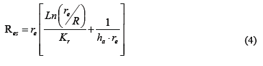
R and re are shown in Fig. 6.
To determine the coefficients of effective convection, we assumed the same values for hHM and hPH, and we perform the next iteration inside the furnace: we calculate the three temperatures, TP, TH and TM with eq. (1)-(3), and then the values of hHM and hPH were recomputed according to eq. (5)-(9) listed below. The three temperatures were recomputed with the new values of hHM and hPH, until that the temperature values do not change with further calculation.
3.2. Temperature profile
After determining the temperatures on the jaws and the walls of furnace, we proceeded to simulate the temperature profile inside the furnace by means of the balance of heat, eq. (10), and its boundary conditions, eq. (11)-(12). In this heat balance, it was assumed that the system is closed, with axial symmetry, without variation in the angular direction and steady state. The control volume considered is the space confined by the inner wall of the tubular furnace and half the height between the jaws (z = Z/2). The origin is considered to be at the center of one of the jaws (see the yellow box in Figs. 2 y 6). The system of equations (eq. 10-12) is solved by finite difference, applying the algorithm of Thomas, where TP, TM, and THwere already calculated with the eq. (1)-(3) and T|Z = 0was determined with eq. (13).

K is the thermal conductivity of the air inside the furnace, according to Kreith [19].
Petter et al. [20], Torrent et al. [21] and Obregon et al. [15] have already used the eq. (10), heat balance, to determine the profile of temperature of a gas confined in a cylindrical geometry.
The values considered for the boundary conditions were: along the axis of the furnace the temperature takes the minimum values (eq. 11) and the temperature in the vicinity of the wall of the furnace is approximate to the temperature on the furnace wall (eq. 12).
The temperature inside the furnace, when the jaws are closed (Z = 0), was determined by the balance of eq. (13).
The heat balance (eq. 10) takes into account the transfer of heat due to velocity and temperature profiles inside furnace.
The velocity profile inside the furnace was determined using the relationship of Navier-Stokes (eq. 14) in cylindrical coordinates, the state equation of an ideal gas and as a boundary condition it was assumed that the velocity is zero at the walls of the furnace, and it presents a maximum on the axis. This boundary condition has been used by Torrente et al. [2] and Cuadrado et al. [26].
The value considered for viscosity, h, in the equations (10) and 14, is 0.0000175 [g/mm*s].
The Navier-Stokes Equation (eq. 14) has been used to determine velocity in free convection furnaces, for example, in research conducted by Gomez et al. [16], Courtin et al. [18], Lee et al. [17], Cawley et al. [14], and Obregón et al. [15] .
To solve the differential equation (eq. 14) we used the finite difference method and with the state equation of ideal gas and its boundary condition, we obtained three tridiagonal matrices. These three tridiagonal matrices were resolved simultaneously with the Thomas Algorithm to obtain the three components of the velocity profile.
4. Simulation results
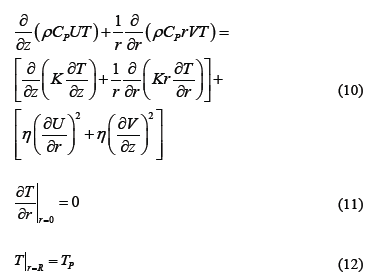
The results of the simulation in Figs. 7, 8 and 9 show that the temperature inside the furnace is not uniform, being colder near the refrigerated jaws (height = 0 mm) and at the axis of the furnace (radius=0 mm) and warmer near the walls of the furnace (radius=25 mm).
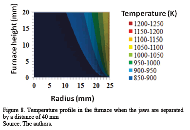
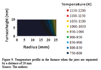
Fig. 7 shows that the highest temperature of the furnace is recorded at a height of 40 mm and a radius of 25 mm, just right on the inner wall of the furnace. This same figure also shows that at a height of 40 mm, right in the middle of the two jaws, there is a difference in temperature of 119 K between the center (around 1113 K) and the wall of the furnace (approximately 1232 K); in the vicinity of the jaws it is observed that the difference in temperature between the same points is similar. The difference observed between the furnace inner walls toward its interior becomes more abrupt in the vicinity of the jaws (height = 0 mm), because the temperature on walls of the furnace was assumed to be constant and the jaws are refrigerated.
When the jaws move towards the inner of the furnace, the temperature inside it decreases as might be expected, since a cooled body is being introduced inside the furnace (Figs. 8 and 9).
Another feature that can be seen by comparing Figs. 8 and 9 with Fig. 7, is that as the jaws advance towards the inside of the furnace, the difference in temperature between the furnace wall and the center increases, from a difference of 119 K, with 80 mm clearance between the jaws, to 350 K and 400 K, for 40 mm and 20 mm of separation, respectively; this is also appreciated in experimental measurements, although in lesser magnitude (see Figs. 3, 4 and 5). This discrepancy is because the simulation determines the temperature of the furnace and not the temperature measured by the thermocouple, for which the heating by radiation experimented by the thermocouple must be considered; this correction can be seen in eq. (15).
Boundary conditions similar to those used in this work, were used by Paulsen et al. [12] in their investigation, in which the temperature of the wall of the heating cylinder was 100°C and the temperature the gas at the entrance of the heating cylinder was at room temperature. It is worth noting that their heating system was used for a different function, as an organic particle nebulizer. Without neglecting the differences in the magnitudes of temperature between the work of Paulsen et al. [12] and this study, the behavior of temperature profiles determined in both studies (Figs. 7, 8 and 9) are very similar.
Hipolito [22] in his thesis also presented two-dimensional temperature profiles, this time for a cylindrical furnace used in pyrolysis for biomasses. The behavior of the temperature profile in his work is also similar to those obtained in this work, with the difference that the furnace of Hipolito [22] was considered opened, with a slight current of ambient temperature air entering the furnace. His conclusions are consistent with the results obtained in this work: as it moving away from the ends of the furnace, the decrease of the temperature in the radial direction is less abrupt. Hipolito [22] determined these profiles using ANSYS FLUENT CFD®. In this work the simulation was conducted in finite difference, generating the mesh with the Thomas algorithm and using Visual Basic.
5. Experimental comparisons
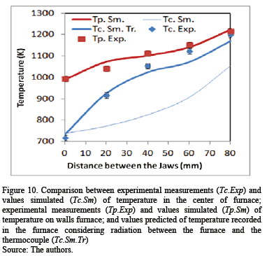
To compare the simulated values of temperature inside the furnace with those measured experimentally, it was necessary to estimate the temperature that the thermocouple should have registered, TTr (Tc.Sm.Tr in Fig. 10), due to radiation between the furnace and the thermocouple, with Tc= T|z=L/2, r=0, from eq. (15) [19].
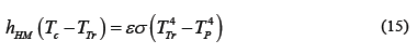
The value considered for emissivity, e, in the eq. (15), is 0.7. This value for oxidized steel is between 0.6 and 0.95 [24]
The simulated values of the temperature in the center of furnace (Tc.Sm) were compared with the corrected values of temperature (TTr in eq. 15) that should be recorded by the thermocouple (Tc.Sm.Tr) and those measured experimentally (Tc.Exp). These values are presented in Fig. 10.
It is important to note that theoretically the temperature in the center of the furnace (T|z=L/2;r=0=Tc.Sm.) is not the same that can be registered with a thermocouple (Tc.Sm.Tr), and this difference increases with the separation between jaws. This difference is minor when the jaws are in the center of the furnace (see Fig. 10). The differences between the simulated values and the experimental measurements of temperatures inside the furnace were expected, because in the simulation we calculated only the temperature of the air inside the furnace (T in eq. 10). However, the thermocouple inside the furnace is heated by radiation from the electric resistance at the furnace wall, therefore, the temperature of the thermocouple is higher than the air inside the furnace, (eq. 15).
Fig. 10 shows that the difference between the temperatures simulated in the center (Tc.Sm) and on the wall (Tp.Sm.) of the furnace is greater when the jaws are separated from each other.
The temperature values obtained from the simulation are close to experimental measurements (see Fig. 10), taking into account the assumptions that were used to simplify calculations in the simulation: steady state, closed system, continuous power of 550 Watts to the resistance, and that the temperature of the jaws and the coefficient of effective convection are uniform.
When comparing the values of temperature of the furnace wall measured experimentally (Tp.Exp. Fig. 10) with those obtained theoretically in the simulation (Tp.Sm. Fig. 10), it can be seen that only at a point, at 20 mm separation between the jaws, the results of the simulation are 33.11 K above the value measured experimentally, which represents an error of 3.18%; in all other cases, the simulation results predict satisfactorily the experimental values.
In the case of temperatures in the center of the furnace, the prediction of the simulations, when radiation between the furnace and the thermocouple is considered, is satisfactory up to 40 mm separation of the jaws, from there, the difference between the experimental and simulated values (which the thermocouple should register) increases. Over 40 mm of clearance between the jaws, the maximum discrepancy was found to be as 60 mm of separation, the temperature recorded experimentally (Tc.Exp. Fig. 10) being 50.76 K greater than what the thermocouple should register (Tc.Sm.Tr Fig. 10), which is equivalent to a maximum error of 4.73%.
Based on these results, the proposed simulation could be a useful tool to predict, with an acceptable approximation, the temperature of compression test specimens up to 40 mm length and diameters smaller to 26.67 mm, according to the standard ASTM E209 [23].
6. Conclusions
In the heating system for hot compression testing, jaws should be refrigerated in order to maintain the temperature in the load cell within its operating range. This produces heat loss by the jaws and makes the values of temperature in their vicinity lower than in the rest of the furnace. This behavior generates a peculiar temperature profile inside the furnace, the temperature being lower in the center than on the walls. When the jaws are farther from the center of the furnace, the temperature in its interior will be greater and the decrease in temperature in the radial direction will be less.
The simulation that is proposed in this paper represents a useful tool which can be used to estimate, with an acceptable approximation (less than the 4.73% error), the temperature inside the furnace during hot compression tests.
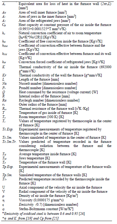
Nomenclature
Acknowledgment
The authors would like to thank the Dean of Research and Development of the Universidad Simon Bolivar (DID), the Laboratory E, Eng. Luis Sanoja and Prof. Armando Blanco.
References
[1] Kalpakjian, S. y Schimd S. R., Manufactura, ingeniería y tecnología, Mexico, Pearson Educación, 2008. [ Links ]
[2] Torrente, G., Torres, M. y Sanoja, L., Efecto de la velocidad de deformación en la recristalización dinamica de un cobre ETP durante su compresión en caliente con temperatura descendente, Rev. Metal. Madrid., 47 (6), pp 485-496, 2011. [ Links ]
[3] Wang, Y., Zhou, Y. and Xia, Y., A constitutive description of tensile behavior for brass over a wide range of strain rates. Mater. Sci. Eng. A., 372, pp. 186-190, 2004. [ Links ]
[4] Jin, N., Zhang, H., Han, Y., Wu, W., and Chen, J., Hot deformation behavior of 7150 aluminum alloy during compression at elevated temperature, Mater. Charact., 60, pp. 530-536, 2009. [ Links ]
[5] Kolmogorov, A., A statistical theory for the recrystallisation of metals, Izv Akad Nauk SSSR, Ser. Matem., 3, pp. 355-359, 1937. [ Links ]
[6] Luton, M. and Sellar, C., Dynamic recrystallization in nickel and nickel-iron alloys during high temperature deformation, Acta. Metall., 17, pp. 1033-1043, 1969. [ Links ]
[7] Cabrera, J. M., Omar, A. y Prack, J., Simulación de la fluencia en caliente de un acero microaleado con un contenido medio de carbono. II parte. Recristalización dinámica: Inicio y cinética, Rev. Metal. Madrid, 33, (3), pp. 143-152, 1997. [ Links ]
[8] García, V., Wahabi, M., Cabrera, J.M., Riera, L. y Prado, J. M., Modelización de la deformación en caliente de un cobre puro comercial, Rev. Metal. Madrid, 37, 2001, pp. 177-183. [ Links ]
[9] Omar, A., Chenaoui, A., Dkiouak, R. y Prado, J. M., Aproximación al control de la microestructura de dos aceros microaleados con contenido medio de carbono en condiciones de conformado en caliente, Rev. Metal. Madrid, 42, pp. 103-113, 2006. [ Links ]
[10] Sanoja, L., Estudio experimental de la recristalización dinámica del cobre durante compresión en caliente, Tesis, Departamento de Ciencia de los Materiales, Universidad Simón Bolívar, 2011. [ Links ]
[11] Zhao, X.L., Ghojel, J., Grundy, P. and Han, L. H., Behavior of grouted sleeve connections at elevated temperatures, Thin-Walled Struc., 44 (7), pp. 751-758, 2006. [ Links ]
[12] Paulsen, D., Weingartner, E., Alfarra, M.R. and Baltensperger, U., Volatility measurements of photochemically and nebulizer-generated organic aerosol particles, J. Aerosol Sci., 37 (9), pp. 1025-1051, 2006. [ Links ]
[13] Ahanj, M., Rahimi, M. and Alsairafi., A., Heat Mass Transfer, CFD modeling of a radiant tube heater, Inter. Commun., 39 (3), pp. 432-438, 2012. [ Links ]
[14] Cawley, M. and Mcbride, P., Flow visualization of free convection in a vertical cylinder of water in the vicinity of the density maximum, Inter. J. Heat Mass Transfer, 47, pp. 1175-1186, 2004. [ Links ]
[15] Obregon, S., Molina, V. y Salvo, N., Simulación de conveccion natural en recintos cerrados, Av. Energ. Renov. Medio Ambient., 9, pp. 885-890, 2005. [ Links ]
[16] Gomez, R., Determinación de un perfil de temperatura de un horno de mufla mediante COMSOL 3.2, Tesis, Universidad Autónoma del Estado de Hidalgo, Mexico, 2007. [ Links ]
[17] Lee, A., Numerical investigation of the temperature distribution in a industrial oven, Thesis, Faculty of Enginnering and Surveying, University of Southern Queensland, Australia, 2004. [ Links ]
[18] Courtin, S., Simulacion bidimencional de la conveccion natural en cavidades cuadradas de paredes horizontales perfectamente conductoras con alto numero de rayleigh, Tesis, Facultad de Ciencias Físicas y Matemáticas, Universidad de Chile, Chile, 2006. [ Links ]
[19] Kreith, F., Principios de Transferencia de calor, Herrero Hermanos Sucesores S. A., Mexico, 1970. [ Links ]
[20] Kaczmarski, K., Kostka, J., Zapat;a, W. and Guiochon, G., Modeling of thermal processes in high pressure liquid chromatography: I. Low pressure onset of thermal heterogeneity, J. Chromatogr. A, 1216 (38), pp. 6560-6574, 2009. [ Links ]
[21] Torrente, G., Puerta, J. and Labrador, N., Two-temperature single flow modelo of a thermal plasma reactor in fluidized bed sisted by magnetic mirror, Phy. Scr., T131, pp. 1-5, 2008. Available at: http://iopscience.iop.org/1402-4896/2008/T131/014010/pdf/1402-4896_2008_T131_014010.pdf [ Links ]
[22] Hipólito, H., Caracterización y modeloamiento del perfil de temperatura al interior de un horno de pirolisis para biomasa, Tesis, Facultad de Minas,Universidad Nacional de Colombia, Sede Medellin, Colombia, 2009. [ Links ]
[23] ASTM, Standard E-209-00, Standard practice for compression tests of metallic materials at elevated temperatures with conventional or rapid heating rates and strain rates, 03.01, ASTM International, 2010. [ Links ]
[24] RAYTEC, Emissivity values for metals [view, 02/04/2014]. Available at: http://www.raytek.com/Raytek/enr0/IREducation/EmissivityTableMetals.htm [ Links ]
[25] DeHoff, R, Thermodynamics in materials science, Second Edition, Taylor and Francis Group, 2006. [ Links ]
[26] Cuadrado, I., Cadavid, F., Agudelo, J. y Sánchez, C., Modelado de flujo compresible unidimensional y homoentropico por el método de volúmenes finitos, DYNA, 75 (155), pp. 199-210, 2008 [ Links ]
G. J. Torrente-Prato, received the Bs. Eng in Material Engineering in 2000, the MSc degree in Material Engineering in 2004, and the PhD degree in Engineering in 2009, all of them from the Universidad Simon Bolivar. Caracas, Venezuela. He is Professor in the Mechanical Department, Universidad Simón Bolívar. His research interests include: simulation and modeling of fluids and solids.
M. Torres-Rodríguez, received the Bs. Eng in Material Engineering in 1986 and the MSc degree in Material Engineering in 1991, all of them from the Universidad Simon Bolivar. Caracas, Venezuela. She is a Full Professor in Mechanical Department of the Universidad Simon Bolivar. Her research interests include mechanical properties and manufacturing processes.
