http://dx.doi.org/10.15446/dyna.v81n188.41275

Flatness-based fault tolerant control

Control tolerante a fallas basado en planitud

 

César Martínez-Torres ^a, Loïc Lavigne ^b, Franck Cazaurang ^b, Efraín Alcorta-García ^a & David A. Díaz-Romero ^a

 

^a Universidad Autónoma de Nuevo León, Nuevo León, México., efrain.alcortagr@uanl.edu.mx
^b Université Bordeaux I, Bordeaux, Francia.,loic.lavigne@ims-bordeaux.fr, franck.cazaurang@ims-bordeaux.fr

 

Received: December 18^th, 2013. Received in revised form: March 10^th, 2014. Accepted: September 18^th, 2014

 

---

Abstract
This paper presents a Fault Tolerant control approach for nonlinear flat systems. Flatness property affords analytical redundancy and permit to compute the states and control inputs of the system. Residual signals are computed by comparing real measures and the computed signals obtained using the differentially flat equations. Multiplicative and additive faults can be handled indistinctly. The redundant signals obtained with the differentially flat equations are used to reconfigure the faulty system. Feasibility of this approach is verified for additive faults in a three tank system.

Keywords: Fault tolerance, differential flatness, three tank system.

Resumen
Este artículo presenta un método de control tolerante a fallas para sistemas no lineales planos. Las propiedades intrínsecas de los sistemas planos generan redundancia analítica y permiten calcular todos los estados y las entradas de control del sistema. Los residuos son calculados comparando las medidas reales provenientes de los sensores y las señales obtenidas gracias al conjunto de ecuaciones del sistema plano. Fallas multiplicativas y aditivas se pueden manejar de manera indistinta. Las señales redundantes obtenidas con las ecuaciones del sistema plano son usadas para reconfigurar el sistema con falla. La factibilidad del método propuesto es verificada para fallas aditivas en un sistema de tres tanques.

Palabras clave: Tolerancia a fallas, planitud diferencial, sistema de tres tanques.

---

 

1. Introduction

Since early in the 90's, Fault Tolerant Control (FTC) algorithms become an active research area due to the importance of operate reliable and/or profitable production systems, see for instance [1]. FTC system means that if a fault occurs in a system, the control system could be capable of overcome the fault effect and continue working (sometimes in a degraded mode). In the frame of analytical redundancy (in contrast with physically redundancy), FTC could be achieved basically in two known ways: The first one considers into the control design the possible effect of faults on the system. This approach is denominated passive and it has a close relationship to robust control design [2]. As it is well known, as far as more faults are considered in the design, the performance of the controller becomes conservative, i.e. the performance is degraded. The second one uses a different strategy: the FTC-algorithm responds to a system fault by modifying the control loop. This approach is denominated active and the main characteristic is the high performance that could be reached [1]. Furthermore, active FTC could cover a larger span of faults.

There are not too much results reported in the literature considering flatness based approach. An early FTC flatness-based approach has been considered in [3], where the fault tolerance is carried out by using the fault estimation (using an algebraic estimation approach). Such estimates are obtained using the differentially flat equations to compute a fault-free version of the states and then compare them versus the faulty sensor. Such operation will provide an estimate of the fault. The approach is intended for actuator faults. According to the authors additive and multiplicative faults could be treated indistinctly. In [4] is presented an approach based also on fault estimation, which is obtained using the differentially flat equations to compute a fault-free version of the states and then compare them versus the faulty sensor. Such operation will provide an estimate of the fault. Then the signal is conditioned using B-splines. The obtained trajectory is subtracted from the measure of the faulty sensor. Only sensor faults are taken into account. This approach is applied to linear systems with a focus on sensor faults. The main disadvantage of both techniques is the fact that estimation plus signal conditioning could take some time to be accomplished. Such time delay could lead the system to instability.

This work presents a FTC flatness-based approach which overcome the time delay of early approaches, the analytical redundancy needed to compute the residual signals is obtained from the inherent properties of the flat systems, in fact if a linear or nonlinear system is flat each state and control input could be expressed as function of a so-called flat output vector, this property will provide the redundancy needed to compute the residual signals. Furthermore a fault-free version of the states and control inputs which are not part of the flat output vector is computed, such reference is the used to hide recover the faulty system. For sensors additive faults are considered in both stages FDI and control reconfiguration, however for faults affecting control inputs only FDI is considered, the fault effect is rejected by the controller.

This paper is organized as follows: section 2 presents the differential flatness property and the flatness motion planning. The FTC approach is presented in section 3. Section 4 presents the results of the proposed approach applied in a classical three tank system, thanks to its versatility this system is widely used in the FTC community, see for instance [5-7]. Section 5 is devoted to present the conclusion.

 

2. Differential flatness

The flatness theory search to determine if a system of differential equations could be parameterized by arbitrary functions. The first works have been carried out in [8], aiming aeronautical applications. The theory development continued in the PhD. dissertation of P. Martin [9], this work has led to the formal concept of flatness presented by M. Fliess et al. in [10].

The differential flatness of non-linear and linear systems could be described by using mathematical formalisms, and specifically differential algebra or differential geometry.

A non-linear or linear system is flat if there exists a set of variables differentially independent, called flat outputs, whose number is equal to the quantity of control inputs, such as, the vector state and the control inputs can be expressed as functions of the flat outputs and a finite number of its time derivatives. By consequence, state and control inputs trajectories can be obtained by planning only the flat output trajectories, this property can be particularly exploited on trajectory planning, see [11-14] and trajectory tracking [15,16]. Flatness could be used to design robust controllers, see for instance [17,18].

Definition 1: Let us consider the nonlinear system 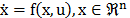the state vector, the control vector and a function of and . The system is differentially flat if, and only if, it exists a flat output vector such as:

• The flat output vector is expressed as function of the state and the control input and a finite number of its time derivatives.

• The state and the control input are expressed as functions of the vector and a finite number of its time derivatives.

Where denotes the time derivative of .

2.1. Flatness-based motion planning

The goal of motion planning is to find control actions that move the concerned system from a start state to a goal condition, while respecting constraints and avoiding collision. Differential flatness is especially helpful to this, because if nominal trajectories for the flat outputs are available it is possible to find open-loop control inputs to drive the system to the final condition. If the nonlinear system is not flat create such trajectories requires an iterative solution by numerical methods. This iterative process can be solved by using optimal control techniques, however for nonlinear systems some problems still unsolved. Besides this solution needs to integrate the system equations in order to evaluate the solution proposed.

Motion planning by flatness, does not need to integrate the system equations and for a flat output trajectory, command inputs can be computed directly, the vector resultant always respect the system dynamics, see eq. (3). By consequence the solutions of the set of differential equations are found. See [11,19].

Definition 1 implies that every system variable can be expressed in terms of the flat outputs and a finite number of its time derivatives. By consequence if we want to compute a trajectory whose initial and final conditions are specified, it suffices to construct a flat output trajectory to obtain the open loop control inputs satisfying the system output desired. In order to compute all the system variables, the flat output trajectory created needs to be at least times differentiable, where is the maximal time derivative of the flat output appearing in the differential flat equations. Additionally this trajectory is not required to satisfy any differential equation. By consequence the flat outputs trajectories can be created by using a simple polynomial approach. If the trajectories needs to be optimal in some sense, a more advanced trajectory generation technique has to be used, some application examples can be found in [11,12,14,20].

 

3. Fault tolerant control approach

The FTC proposed approach presented in Figure 1 keeps the nominal control in order to reduce the time response after a fault, the idea is to couple the FDI stage together with the fault recovery strategy, in fact some signals used to compute the residues are not affected by the fault, by consequence those signals are used to response to the fault effect.

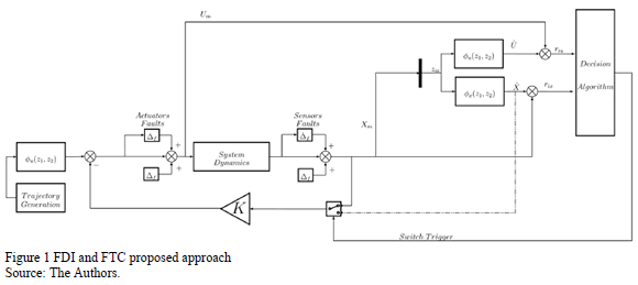
3.1. Fault Detection and Isolation

Let us consider a nonlinear flat model of dimension , and control inputs, with as first set of flat outputs, which corresponds to components of the state vector, also suppose that the full state is measured, it is always possible to compute residues:

• State residues, because the full state is supposed to be measured.
• Control inputs residues.

The residual signals are computed as follows:

where and are the and measured state and control input respectively and and are the and state and control input calculated using the differentially flat equations. Suppose that we have a nonlinear system composed by four states, and two control inputs , as depicted in definition 1, the number of control inputs are equal to the number of flat outputs, by consequence , suppose too that the nonlinear system is flat, with the flat output vector equal to .

This stage can be improved if a second set of flat outputs is found, see [21] for further details.

3.1.1. Residues computation and fault recovery

The proposed approach has the next consequences:

• The maximal number of residues is four.
• Sensor faults not affecting flat outputs can be isolated depending on the system.
• Flat output sensor faults can be detected but cannot be isolated.

The residual signals are computed as follows:

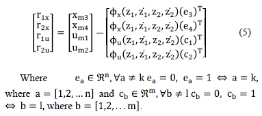
Analyzing the eq. (5) it is straightforward to see that if a fault affects the state measure of , the residual will be affected, the rest of residues are independent of this measure, so they will not be affected by the fault. A fault affecting or the control inputs can be analyzed in the same manner.

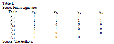
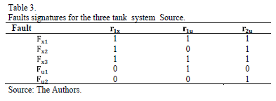
When a fault affects one of the flat outputs, all the residues will be affected, by consequence the fault can be detected but it cannot be isolated. The Table 1 presents each fault signature.

Fault isolation is assured for each state not included in the flat output vector, additionally the flat outputs are considered fault-free at any time, as consequence the right part of the eq. (5) will be fault-free at any time, such reference is then used to recover the system after the fault. The controller reference is changed by a switch, which is triggered by a decision algorithm.

Fig. 2 presents the control reconfiguration proposed approach, in this, the nominal trajectory is calculated by creating trajectories for each flat output and then, using the eq. (3) to compute the nominal control inputs. Additive and multiplicative faults are consider for both, sensors and actuators. In order to create the residual signals (eq.(4)), each flat output needs to be measured, such measure is then introduced in eq. (2) and (3), by consequence control inputs and states estimations are available, such estimations are helpful to recover the system after fault by simply changing the faulty measure for the estimated one.

Let us retake the example presented previously. If a fault affects the measure signal , the fault will be detected and isolated, see Table 1. Considering that the flat output vector is compound by and such states are consider fault-free at any time, an unfaulty reference of can be estimated using the right part of the eq. (5), such reference is then used to feed the controller and recover the system.

3.2. Derivatives estimation

In order to compute the system states and the control inputs of the system, and consequently the residual signals, the time derivatives of the flat outputs of the system has to be estimated.

In this work a high-gain observer [22] is used to evaluate the time derivative of noisy signals. In order to improve the performance of the high-gain observer, a low-pass filter is synthesized. The delay introduced by the filter could affect the control reconfiguration; by consequence especially attention on its design has to be considered.

3.3. Detection robustness

For this work the fault detection is achieved by simply comparing the residual amplitude versus a fixed detection threshold. The amplitude of the detection threshold is fixed by running series of fault-free simulations of the system. Three different simulations are run, the first one by changing each parameter individually in the same percentage upwards and downwards. The two final simulations are run by varying all the parameters plus and minus the same percentage used in the previous simulation.

Finally, the amplitude of the detection threshold is fixed by selecting the worst case among all the results of the simulations, plus a security marge. Such marge is added in order to avoid false alarms caused by the unknown perturbations or modeling errors.

 

4. Three tank system

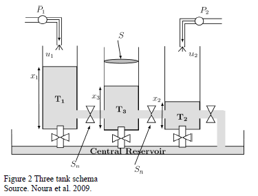
The proposed approach is applied to a classical three tank system; this classical system is used such system is composed by three tank, a central reservoir and two pumps in charge of introduce liquid to the system. Each tank is linked to the central reservoir by means of a pipe with transversal section equal to S. The tanks are linked between them with a pipe with the same section. See Fig. 2.

The nonlinear mathematical model is obtained as follows:

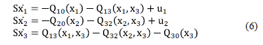
Where, x_i, i=1,2,3, denotes the individual tank; Q_i0, i=1,2,3 represents the outflow between each tank and the central reservoir, Q₁₃ and Q₃₂ are the outflow between tank one and tank three and the outflow between tanks three and two respectively, u₁ and u₂ are the incoming flows of each pump.

The valves connecting tanks one and three with the central reservoir are considered closed, so Q₁₀ and Q₃₀ are always equal to zero.

The flows Q₁₃, Q₃₂ and Q₂₀ can be expressed as follows:

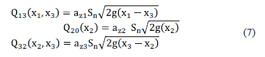
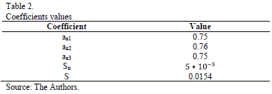
Where S_n represents the transverse section of the pipes connecting the tanks and a_zr, r=1,2,3 represents the flow coefficients. Coefficients values are depicted in Table 2.

4.1. Flat model

A system is flat if and only if each state and control input is expressed in function of the flat output, see definition 1 for more details. Let us define the flat output vector as: , the differentially flat equations can be written as follows:

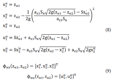
It is straightforward to see that the three tank system is flat, eq. (8) prove that each single state, and the two control inputs can be written as a function of the flat output vector and a finite number of its time derivatives. Eq. (9) groups such functions in a vector, in order to simplify the notation.

4.2. Fault Detection and Isolation

Additive faults affecting level sensor and flow actuators are considered. For such faults, a +10cm measure error is considered in sensors and an extra flow of is added to input flows. Only a single fault may be present at a time, once the fault appears (at 100 s) it is recurrent until the end of the simulation.

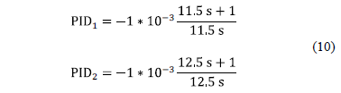
Two PID controllers are connected to high measures of tanks one and two, see (10). Such controllers are synthetized by making a compromise between the fault rejection dynamic and the noise level presented in the measurements. As described previously faults are detected by simply comparing the residual signal amplitude versus the threshold amplitude. The detection threshold was defined by changing the flow parameters in the range of 10%; afterwards the maximal value for each residue (positive and negative) plus an error margin is used as the final amplitude of the detection threshold. This margin adds robustness and avoids false alarms, if a residue exceeds the threshold, such residue is taken into account to construct the fault signature and by consequence isolate the fault.

Flat outputs trajectories were generated by using a fifth order polynomial. White noise is added to the measured outputs. Derivatives are estimated by using a high-gain observer [22] coupled to a low-pass filter to reduce the amplitude of the noise and improve the derivative estimation.

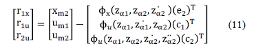
According to the process described in section 3.1.1 the residuals are obtained by computing the difference between the value given by the measuring sensor and the estimated

value obtained with the differentially flat equations, eq. (8) and eq. (9). Equation (11) presents the three residuals.

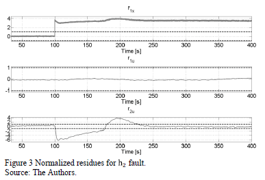
The results are consistent with the analysis presented in section 3.1.1. Let us analyze for instance the fault of the high measure of tank number two. Looking in detail the eq. (11) it is straightforward to see that the residue is the only one depending of the measure , by consequence, this residue is affected, however, since the feedback controller is connected to this measure , the pump number two, which is directly connected to this tank reacts to the fault as well, by consequence the residue is affected too. See Fig. 3.

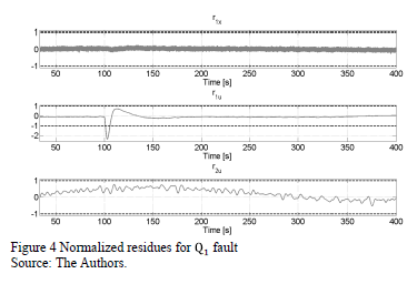
Faults affecting flow pumps could be analyzed in the same manner, for instance a fault affecting the measure of the pump number one affects directly the residue . Due to the fact that we work in closed loop the residue is affected too but in a smaller quantity, such amplitude variation is not enough to exceed the threshold and by consequence this is not taken into account to construct the fault signature, see Fig. 4.

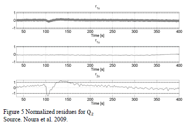
For a fault in pump number two the residue affected directly is the residual signal , for this case and since in the three tank system the high level of the two other tanks depends of the high measure of tank number one the pump one increase its flow and by consequence the measure of the first tank is affected, but the amplitude is not enough to exceed the threshold, see Fig. 5.

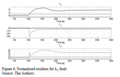
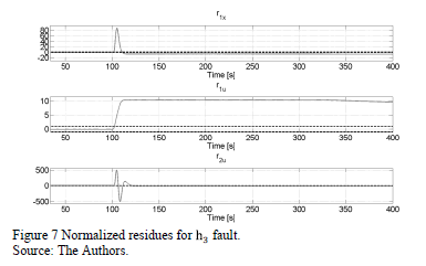
As expected for an individual fault affecting the measures of the flat outputs the three residues are triggered, by consequence each individual fault can be detected but it is impossible isolate them by simply comparing the fault signature, see Figs. 6 and 7. However none of the PID is connected to the measure of tank three, so this fault will not affect the final position, this results in a non-optimal isolation between faults in tank one and tank three. By this way every sensor and actuator fault can be detected and isolated. Table 3 presents a summary of the residues triggered by each fault.

All the residual signals are normalized between 1 and -1; the boundaries are the maximal and minimal value of the threshold.

4.3. Control reconfiguration

Once the fault is detected the signal measure is changed by switching between this and the one computed with the differentially flat equations eq. (8).

Fig. 8 shows the position error between nominal trajectory and trajectories with control reconfiguration and without reconfiguration. It is straightforward to see that in case of not reconfigure the controller the error is bigger and permanent, however for the reconfiguration case the error is close to zero at the end of the simulation.

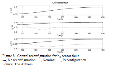
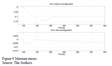
Fig. 9 presents the errors for the final position of the tank number two in the two cases, with and without reconfiguration; it is clearly to see that if the control reconfiguration is not carried out the final trajectory is not followed.

Actuators faults are compensated by the controller, tank three sensor fault does not affect the final position and faults affecting water level measure of tank one can be isolated, but a non-faulty measure is not available. By consequence if such fault affects the system, the system cannot be reconfigured.

 

5. Conclusions

This paper presents a flatness-based Fault Tolerant Control approach. The feasibility of the proposed approach is investigated in a classical three tank system. For this particular system faults affecting actuators are detected. The fault affecting the high measure sensor of tank number two is detected and isolated by simply comparing the amplitude of the residual signal versus a threshold, additionally thanks to the properties of the flat systems a fault-free version of the measure is estimated, such signal is then used to recover the system after the fault.

Actuators faults are detected and isolated in the same manner. Active reconfiguration is not considered since those faults are rejected by the controller.

Faults affecting the flat outputs can be detected but cannot be isolated using the threshold-based approach, however since the state feedback controller does not depend of the measure of tank three this fault will not impact the final position, contrary of the fault measure of tank number one, as consequence this result in a non-optimal identification between such faults. This can be avoided if as in [23] a second set of flat outputs is found, by this way not only one but two redundant signals are available for reconfiguration purposes, see [23] for further details.

 

Acknowledgment

The fourth author thanks CONACYT Mexico for the financial support through the grant 178282-CB-2012-01.

 

References

[1] Isermann, R., Fault-diagnosis systems: An introduction from fault detection to fault tolerance, Springer, 2006. http://dx.doi.org/10.1007/3-540-30368-5        [ Links ]

[2] Benosman, M., Passive fault tolerant control, robust control, Theory and applications, [Online] Available from: http://www.intechopen.com/books/robust-control-theory-andapplications/passive-fault-tolerant-control, 2011.         [ Links ]

[3] Mai, P., Join, C., Reger, J. et al., Flatness-based fault tolerant control of a non-linear MIMO system using algebraic derivative estimation, in: 3rd IFAC Symposium on System, Structure and Control, SSC'07, 2007.         [ Links ]

[4] Suryawan, F., De Dona, J. and Seron, M. Fault detection, isolation, and recovery using spline tools and differential flatness with application to a magnetic levitation system, in Control and Fault-Tolerant Systems (SysTol), 2010 Conference on, IEEE, pp. 293-298, 2010        [ Links ]

[5] Noura, H., Theilliol, D., Ponsart, J.C. and Chamseddine, A., Fault-tolerant control systems: Design and practical applications, Springer, 2009. http://dx.doi.org/10.1007/978-1-84882-653-3        [ Links ]

[6] Adam-Medina M., Theilliol, D., Astorga-Zaragoza, C.M., Guerrero-Ramírez, G. and Vela-Valdés, L.G., Diagnostico de fallas basado en un filtro desacoplado para sistemas no lineales representados por un enfoque multi-modelos, DYNA, 77 (162), pp. 313-323, 2010.         [ Links ]

[7] Köppen-Seliger B., Alcorta-García, E. and Frank, P.M., Fault detection: different strategies for modelling applied to the three tank benchmark-a case study, Proceedings of European Control Conference, 1999.         [ Links ]

[8] Charlet, B., Lévine J. and Marino, R., Sufficient conditions for dynamic state feedback linearization, SIAM Journal on Control and Optimization, 29 (1), pp. 38-57, 1991. http://dx.doi.org/10.1137/0329002        [ Links ]

[9] Martin, P., Contribution à l'étude des systèmes différentiellement plats, PhD. Thesis, École des Mines, Paris, France 1992.         [ Links ]

[10] Fliess, M., Lévine J., Martin, P. and Rouchon, P., Flatness and defect of non-linear systems: Introductory theory and examples, International Journal of Control, 61n(6), pp. 1327-1361, 1995. http://dx.doi.org/10.1080/00207179508921959        [ Links ]

[11] Louembet, C., Génération de trajectoires optimales pour systèmes différentiellement plats: Application aux manoeuves d'attitude sur orbite, PhD. Thesis, Université de Bordeaux I, Bordeaux, France, 2007.         [ Links ]

[12] Louembet, C., Cazaurang, F. and Zolghadri, A., Motion planning for flat systems using positive B-splines: An LMI approach, Automatica, 46 (8), pp. 1305-1309, 2010. http://dx.doi.org/10.1016/j.automatica.2010.05.001        [ Links ]

[13] Milam, M.B., Franz, R. Hauser J.E. and Murray, R.M., Receding horizon control of vectored thrust flight experiment, IEE Proceedings-Control Theory and Applications, 152 (3), pp. 340-348, 2005. http://dx.doi.org/10.1049/ip-cta:20059031        [ Links ]

[14] Van-Nieuwstadt, M.J. and Murray, R.M., Real-time trajectory generation for differentially flat systems, International Journal of Robust and Nonlinear Control, 8 (11), pp. 995-1020, 1998. http://dx.doi.org/10.1002/(SICI)1099-1239(199809)8:11<995::AID-RNC373>3.0.CO;2-W http://dx.doi.org/10.1002/(SICI)1099-1239(199809)8:11<995::AID-RNC373>3.3.CO;2-N

[15] Antritter, F., Müller B. and Deutscher J., Tracking control for nonlinear flat systems by linear dynamic output feedback, Proceedings NOLCOS 2004, Stuttgart, 2004.         [ Links ]

[16] Stumper, J., Svariceck F. and Kennel, R., Trajectory tracking control with flat inputs and a dynamic compensator. arXiv preprint arXiv: pp. 1211-5759, 2012.         [ Links ]

[17] Cazaurang, F., Commande robuste des systèmes plats application à la commande d'une machine synchrone, PhD. Thesis, Université Sciences et Technologies-Bordeaux I, Bordeaux, France,1997.         [ Links ]

[18] Lavigne, L., Outils d'analyse et de synthèse des lois de commande robuste des systèmes dynamiques plats, PhD. Thesis, Université Sciences et Technologies-Bordeaux I, Bordeaux, France, 2003.         [ Links ]

[19] Morio, V., Contribution au développement d'une loi de guidage autonome par platitude. Application à une mission de rentrée atmosphérique, PhD. Thesis, Université Sciences et Technologies-Bordeaux I, Bordeaux, France, 2009.         [ Links ]

[20] Cazaurang, F. and Lavigne, L., Satellite path planning by flatness approach, International Review of Aerospace Engineering, 2 (3), pp. 123-132, 2009.         [ Links ]

[21] Martínez-Torres, C., Lavigne, L.F., Cazaurang, F., Alcorta-García, E. and Diaz-Romero, D., Fault detection and isolation on a three tank system using differential flatness, in European Control Conference. Zurich, Switzerland, 2013.         [ Links ]

[22] Vasiljevic, L.K. and Khalil, H.K. Error bounds in differentiation of noisy signals by high-gain observers, Systems & Control Letters, 57 (10), pp. 856-862, 2008. http://dx.doi.org/10.1016/j.sysconle.2008.03.018        [ Links ]

[23] Martínez-Torres, C., Lavigne, L.F., Cazaurang, F., Alcorta-García, E. and Diaz-Romero, D., Fault tolerant control of a three tank system: A flatness based approach, in 2nd International Conference on Control and Fault-Tolerant Systems. Nice, France, 2013.         [ Links ]

 

C. Martinez-Torres, obtained his B.Sc degree in Electronics and Communication Engineering from the Universidad Autónoma de Nuevo León (UANL), Mexico; the MSc degree in Aerospace Engineering in 2010, from Bordeaux University, France and the PhD degree in Automatic Control in 2014, from the UANL and the University of Bordeaux. His current research interest is fault tolerance guidance based on flatness approach dedicated to nonlinear systems.

L. Lavigne, obtained his PhD. degree in Automatic Control in 2003 from the University of Bordeaux I, France. Since September 2005 he has been Associate Professor at Bordeaux I University. His main research interests include fault detection and diagnosis, path planning, flat systems and robust control dedicated to aeronautics and space domains. Dr. Lavigne has been involved in two different European projects (GARTEUR, SIRASAS) which deals respectively on robust control and Fault Detection and Diagnosis in the Flight Control System

F. Cazaurang, obtained the BSc and MSc degrees in Electrical Engineering from ENS Cachan in 1988 and 1990, respectively, the PhD. degree in Automatic Control in 1997from University Bordeaux I, France. From September 1992 to August 1998 he worked as lecturer at Bordeaux University. From September 1998 to August 2010 he worked as Associate Professor of Control engineering in Bordeaux University. Since 2010 he has been Professor of Control Engineering in Bordeaux University. His main research interests include path planning, fault tolerant guidance dynamic inversion and robust control dedicated to aeronautics and space domains.

E. Alcorta-García was born in Monterrey, Nuevo León, Mexico in 1968. He received the BSc. degree in Electronics and Communication Engineering in 1989 and the MSc. in Electrical Engineering (Automatic Control) in 1992 from the Universidad Autónoma de Nuevo León (UANL), Mexico and the Dr.-Ing. in Electrical Engineering (Automatic Control) in 1999 from the Univeristy Gerhard Mercator of Duisburg (actually Duisburg-Essen University), Germany. Since November 1999 he has held a teaching and research position at the UANL. His research interests include model-based fault diagnosis, fault tolerant control and observers.

D. Diaz-Romero, received his BSc Eng. and MSc. degrees from Universidad Autónoma de Nuevo León, Mexico and his PhD degree in automatic control theory from The University of Sheffield, U.K. He has worked in industry and academics. He currently holds the position of full time researcher at Universidad Autónoma de Nuevo León, Mexico.