DOI: http://dx.doi.org/10.15446/dyna.v83n197.48134

Assessing the loss-of-insulation life of power transformers by estimating their historical loads and ambient temperature profiles using ANNs and Monte Carlo simulations

Evaluación de la pérdida de vida del aislamiento solido en transformadores de potencia, estimando la historia de carga y los perfiles de temperatura ambiente por medio de redes neuronales artificiales y simulaciones de Monte Carlo

 

Andrés Arturo Romero-Quete, Enrique Esteban Mombello & Giuseppe Rattá

 

Instituto de Energía Eléctrica, Universidad Nacional de San Juan - Consejo Nacional de Investigaciones Científicas y Técnicas. San Juan, Argentina. aromero@iee.unsj.edu.ar, mombello@iee.unsj.edu.ar, ratta@iee.unsj.edu.ar

 

Received: January 5^th, 2015. Received in revised form: October 20^th, 2015. Accepted: March 30^th, 2016.

 

This work is licensed under a Creative Commons Attribution-NonCommercial-NoDerivatives 4.0 International License.

---

Abstract
A non-invasive method useful for asset management is to estimate the functional age of the insulating paper of the transformer that is caused by thermal aging. For this purpose, the hot-spot temperature profile must be assessed by means of some transformer characteristics, the historical load, ambient temperature profiles and a set of equations. In many in-service unit cases, the available data is incomplete. This paper proposes a method to deal with the lack of data. The method is based on the estimation of the historical load and ambient temperature profiles by using an artificial neural network and Monte Carlo simulations. The probable loss of total life percentage of a 30 MVA power transformer is obtained through the proposed method. Finally, the corresponding results for the assessed transformer, a model validation section and conclusions are presented.

Keywords: aging; artificial neural network; asset management; Monte Carlo methods; load profile forecasting.

Resumen
La estimación de la pérdida de vida es útil para la gestión de transformadores de potencia. Un método, no invasivo, es estimar la edad funcional del papel aislante del transformador, mediante las guías de carga. Para esto, el perfil de temperatura del punto caliente es calculado a partir de características técnicas del transformador, los perfiles carga y temperatura ambiente y un conjunto de ecuaciones diferenciales. En la práctica, la información disponible para este análisis es incompleta. En este artículo se presenta un método para estimar la carga histórica y los perfiles de temperatura ambiente experimentados por el transformador, cuando existe falta de datos. Para este fin, el método emplea una red neuronal artificial y simulaciones de Monte Carlo. El método es aplicado a un transformador de potencia de 30 MVA. Los resultados obtenidos son analizados en una sección de validación para finalmente dar las conclusiones del trabajo.

Palabras clave: envejecimiento; red neuronal artificial; gestión de activos, simulación de Monte Carlo; pronóstico del perfil de carga.

---

 

1. Introduction

Power transformers play a fundamental, strategic role in power systems. In power transformer management, it is useful to estimate, as closely as possible, the current condition of the unit. There are several monitoring and diagnostic techniques that aimed to estimate the transformer condition. One of these techniques seeks to assess the loss of total life percentage of the unit's insulating paper, which can be expressed in terms of the functional age resulting from thermal degradation. It is to be noted that the functional age is different from the calendar age of the transformer [1,2].

A transformer aging failure is an irreparable failure that is more probable when the loss of life percentage is approaching 100%. In this regard, this measure is useful to make appropriate decisions, e.g., the design of a Suitable scheme of maintenance to prolong unit life.

In a transformer in service, internal temperatures increase as load and ambient temperature rise, and vice versa. High internal temperatures reduce the mechanical strength of the cellulose insulation as time passes [3]. The Hot Spot Temperature (HST) is a useful measure to estimate the thermal effect of paper-aging. In fact, after developing a transformer post mortem assessment, it was found that HST is a critical factor [4]. HST is a function of load, ambient temperature, and features of the unit.

Consequently, the functional age of the transformer can be roughly assessed through HST estimation. If the historical HST profile, i.e., the data of HST values against time, is available for the whole period of the unit operation, then the thermal aging of the insulating paper can be estimated as described in the IEEE and the IEC loading guides, [5,6]. The formula to assess transformer aging is based on the condition of new paper, and can only be used to calculate the relative paper deterioration. Since the aging equation is based on the HST, and the HST calculation on load data, it is then necessary to have access to the complete loading history of the unit.

However, transformer loading history is not usually well-known in practice. To overcome this drawback, this paper proposes a method to deal with the lack of data. The methodology is founded on the fact that, nowadays, electric networks have Supervisory Control and Data Acquisition (SCADA) systems that allow for the online storage of measured values such as load, date and ambient temperature. Even if a part of this data has not been recorded, e.g., in the period previous to the SCADA implementation, the available data can be used to estimate the unrecorded historical load data.

The estimation of lacking load data relies on the statistical analysis of ambient temperatures and on the identification of historical load features. An Artificial Neural Network (ANN) is then trained in order to estimate the complete loading probable profile. Because the uncertainty in the HST estimation must be modeled, the next step requires Monte Carlo Simulations (MCS) to be performed by using both ambient temperature and loading probable profiles as inputs. Subsequently, the estimated probable HST profiles are used to assess the frequency of occurrence of the functional age of the insulating paper and its percentage loss of life.

For the HST calculation, a recent model that considers oil viscosity in temperature dependence has been used [7-9]. Finally, the probable functional age of the insulating paper and therefore, the loss-of-insulation life percentage of a real power transformer are assessed, the results are discussed, and conclusions are presented from the case study.

 

2. Estimation of functional age and loss-of-life percentage of the insulation paper

2.1. Ageing models

In oil-cooled power transformers, paper is used as one of the insulating materials due to its outstanding characteristics, e.g., excellent dielectric and mechanical properties. Paper is comprised of lignin, hemicellulose and cellulose. The cellulose molecules are built by long chains of glucose rings. The average length of these chains, termed Degree of Polymerization (DP), determines the functional characteristics of the paper, [3].

When paper is exposed to water, oxygen, heat and acids, all of which are aging agents, the long molecular chains are cleaved by chemical reactions. As a consequence, the DP and the expected lifespan of the insulating paper decrease.

The aging agents act simultaneously; consequently, the mathematical modeling of the aging process is very complex, resulting in a non-linear Arrhenius plot. However, for practical purposes most of the researchers and organizations assume independent processes, and as such, the total degradation becomes the sum of degradation from each process that can be described by an individual equation, [3,5]. Annex I in [5], introduces an interesting discussion of the history of loss of insulation life. It also states that each aging agent will have an effect on degradation rate, so they must be individually controlled. Moreover, it is observed that whereas the water and oxygen content of the insulation can be controlled by the transformer oil preservation system, the transformer operating personnel is responsible for the control of heat.

This research is mainly focused on the influence of heat in the aging process. However, it must be recognized that time variations of the other agents could strongly affect the aging speed. Note that as concluded in [10,11], "water is more important than oxygen for transformer aging; and acids are of central significance for understanding the aging of paper and for evaluating the effects of oil maintenance."

This assumption could relate to the transformer in the case study reported here, since in the San Juan Province, Argentina, where the unit operates, the average ambient relative humidity is 48%. Also, as can be observed in references [12,13], there is a direct relation between moisture in air, oil, and insulating paper. The higher the relative air humidity, the higher the moisture uptake rate of the insulating liquids will be, and consequently, that of the paper. Consequently, the influence of moisture for this specific case is lower than that for transformers located in areas with a higher average relative humidity. Nevertheless, to achieve more general results, additional research must be conducted in order to model the moisture influence.

Eq. (1), as written in [5], defines the aging acceleration factor, F_AA, as a function of the HST in the windings, in ºC. The empirical constant 15000 is the aging rate constant that is better described in annex I, contained in [5]. The reference temperature, , coincides with the rated HST, which for thermally upgraded paper is =110 °C.

Eq. allows the functional age of insulating paper to be assessed. This expression is the summation in a determined period of time of the products obtained by multiplying intervals of time, , (with i=1, 2…,n, and n as the number of time intervals for the whole period of time) by its respective computed aging acceleration factor, F_AA,i, for which the insulating paper has been exposed to a given

In , both and n are specified by the load profiles that will later be described in section 4. The functional age, A_F, is then used to calculate the loss-of-insulation life percentage as:

In , is the normal insulation life at the reference temperature, , in hours. The benchmark of normal insulation life for well-dried, oxygen-free 65 °C average winding temperature rise system is reported in [4,14]. A 200 retained degree of polymerization in insulation has been adopted in this article as the normal insulation life criterion, and it corresponds to 150000 hours for =110 °C.

2.2. Hot spot temperature estimation

The functional age, due to thermal aging, depends on the HST. This is because the winding insulating paper ages faster in the region in which the hottest temperature is present. When no fiber-optic sensors are installed inside the transformer, as is the common case in older units, the HST must be estimated through models based on measured oil temperatures [15].

Several HST models, ranging from simple to very complex, have been proposed in the bibliography, [5-9]. The qualitative criteria for selecting a HST model for this study were: i) availability of the technical transformer data and parameters the HST model is based on, ii) performance simulating transient or varying loads with altering ambient temperature, and, iii) top-oil temperature (TOT) based model, which exhibits a suitable performance [16].

A thermal model satisfying most of the above defined criteria is the HST model presented by Susa in [7-9]. In this model, HST and TOT differential equations account for oil viscosity changes with temperature. One advantage of this model is that it is only based on nameplate data and few heat run test protocol parameters. The differential equations for the TOT, , and the HST, , are respectively:

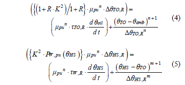
where, R is the ratio of load losses at rated current to no-load losses, K is the load factor and quotient of load over rated load, is the per unit oil viscosity given by the ratio of the current oil viscosity over rated oil viscosity , n is an empirical constant dependent on whether the oil circulation is laminar (n=0.25) or turbulent (n=0.33), m is an empirical constant related with the shape of the thermal curve, is the rated TOT rise over ambient (measured in °C), is the rated HST rise over TOT (measured in °C), is the rated top-oil time constant,is the rated winding time constant in minutes, and is the ambient temperature.

Equations to model oil viscosity variations with temperature are shown in [7-9]. For Oil Natural - Air Natural (ONAN) cooling mode, the value of constants n and m is 0.25. For the Oil Natural - Air Force (ONAF) and Oil Force - Air Force OFAF cooling modes, in power transformers with external cooling these values are n=0.5 and m=0.1.

The winding losses corrected for the HST, , are calculated, as per the following:

where is the ratio of DC losses to total winding losses, is the ratio of winding eddy losses to total winding losses, is the temperature correction factor, 225 for Al and 235 for Cu, and the total winding losses are .

It should be noted that DC losses in are measured by applying a direct current to the windings, whereas eddy losses in the windings are not separately measurable. Furthermore, DC losses are not necessarily given on the nameplates. Nevertheless, Jauregui states in [16] that for load levels near the transformer rated load, (i.e., in a no-overload transformer condition) the winding losses correction is unnecessary. Therefore, if necessary, can be omitted in eq. , which will lead to:

Thus, it can be concluded that the Susa HST model can be simplified for applications where only nameplate data and no heat-run test protocol are available.

2.3. Necessary data to estimate the hot spot temperature

A listing of the transformer data necessary to calculate the HST at time i for the mentioned model includes the following: winding eddy losses, winding resistive losses, DC or I²R losses, load losses, no-load losses, winding-time constant (estimated by means of weight of windings), oil-time constant (estimated by means of the mass of oil), rated TOT rise over ambient temperature, rated HST rise over TOT, rated TOT, rated HST, and both ambient temperature and load at time i. Moreover, selecting appropriate transformer constants requires knowledge of characteristics such as the cooling stages and the winding conductor material. Once the HST is obtained at time i, the procedure must be repeated for the whole operational period of the unit in order to apply and to estimate A_F.

 

3. Problem description and proposed methodology

3.1. Problem description

The aim of this paper is to present a methodology to estimate the functional age, A_F, of insulating paper of aging power transformers when part of data regarding load and ambient temperature profiles for the complete operational period of the assessed transformer is missing.

3.2. Scheme of the proposed methodology

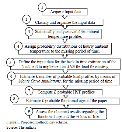
To assess the A_F of the insulating paper, missing historical temperature and load data must be estimated to be able to then apply the models presented in section 3. Taking this into consideration, the following general scheme is proposed as a suitable methodology to address the problem.

In the following section each one of the steps in Fig. 1 will be explained in more detail.

Step 1: Acquire the following input data:

• -Data as described in section 2.3, to thermally model the transformer under study.
• -All available information regarding power delivered hourly through the transformer, and the ambient temperature at the power station; e.g., information acquired by the SCADA.
• -All historical information about ambient temperature and monthly or yearly electric energy consumption in the district in which the power transformer operates.

Step 2: Classify, organize and filter inadequate or atypical data from the hourly load and ambient temperature profiles, acquired in step 1. This step must provide typical values to

Step 3: Analyze the historical ambient temperature statistically. Once the available ambient temperature profile has been preprocessed, normalized days are defined.

For this purpose, each month of available ambient temperature data can be divided into three packages of approximately ten days, i.e., D ≈10. For each package the hourly mean temperature and the standard deviation, s_h, is calculated as:

where d=1,2,..., D, and q_h is the observed temperature at hour h for each day d. Moreover, there is a correlation between adjacent hourly ambient temperatures. To model this dependence, a 24x24 correlation matrix, R_d, is computed for each normalized day. Based on this routine, 24 pairs of and s_h, with h=1,…24, and one correlation matrix R_d are obtained for each normalized day. It is noted that the covariance matrix of the normalized day S_d can also be computed since it is a function of the matrix R_d and the standard deviation vector of 24 elements s_h,d, [16].

Step 4: Assign probability distributions of ambient temperature to the missing period of time. Completing the ambient temperature curve procedure includes assigning one of the obtained normalized days in the previous step to each day in the missing period of time. This action can be performed by comparing features of the normalized days with those known for the days in the missing period, e.g. the Euclidian distance, d, which is given by:

where is a vector containing a pair of values of the historical maximum and minimum daily temperatures for unknown days (i.e., whose hourly temperature profile is unknown) and is a vector containing the same values of a normalized day. These can be used to select the normalized day that exhibits the minimal distance in order to then assign this information to the missing day.

Step 5: Define the input data for the estimation of the historical load and implement a suitable ANN for load forecasting.

References to estimate the historical load were not found; however, load forecasting is a well-known field of work in electrical engineering. In effect, there are various techniques, which have been extensively studied and used in time series forecasting, e.g. Autoregressive Integrated Moving Average (ARIMA) and its variants, Artificial Neural Networks (ANNs), and hybrid methods such as ANNs/ARIMA [18]. However, in this paper ANNs have been selected to deal with the described problem since some researchers have compared and tested this technique, concluding that ANNs could successfully capture the nonlinear relationship between the load and the weather [19]. In effect, ANNs are better suited in terms of ARIMA since the first can capture nonlinear patterns between input and output parameters while the second is limited by the pre-assumed linear form of the model. It must be noted that hybrid methods which combine both ARIMA and ANN are being investigated. Future research could be conducted on this subject to improve the forecasting accuracy; however, this research lies outside the scope of this paper.

In general, an ANN does non-linear curve fitting and is able to find a function to subsequently calculate load values dependent on various input parameters [20]. A two-layer feed-forward network with sigmoid hidden neurons and linear output neurons can fit multi-dimensional mapping problems arbitrarily well if provided with consistent data and enough neurons in its hidden layer [21]. In this network, the information only moves in one direction, forwards, i.e., data goes from the input nodes through the hidden nodes and then to the output node.

Therefore, we selected a feed-forward ANN structure. It basically compares the calculated output value with a desirable result, the target value. The target values are the load values that are stored by the SCADA: in effect, the available load profile. Whereas there is one single output, the load, there are several input parameters. In this approach, the input parameters are the hourly ambient temperatures (Tamb), year, month, weekday, hour and the monthly energy demand (Ed). Fig. 2 illustrates inputs and outputs defined for the ANN.

Step 6: Estimate a quantity of L probable ambient temperature and load profiles by means of Monte Carlo simulations, where L is the number of simulations, for the missing period of time. For this purpose, the probability distributions of ambient temperature defined in step 4, and the input data for the ANN implemented in step 5 are used.

Step 7: Compute L probable HST profiles by using the formulation presented in section 2.2 from the L probable profiles that was computed in steps 4 and 6.

Step 8: Estimate L, probable functional ages of the insulating paper by using formulation presented in section 2.1 from the L HST profiles computed in step 7.

Step 9: Assess the results obtained regarding the A_F from the L probable values computed in step 8, and compute a histogram for the % loss-of-insulation life.

 

4. Case study

In this section, probable HST profiles and a probability density function for the loss-of-insulation life of a 30 MVA and 132 +6/-12 x 1 %/ 34.5/13.8 kV rated step-down transformer will be estimated through the general scheme, shown in Fig. 1. The unit is connected in YN/yno/d11. The rated cooling is ONAN/ONAF at 70/100 % of load. It should be observed that the order to start running the assessed unit fans, i.e. to start the ONAF mode, is given by a commercial temperature monitor.

It is remarkable that there have been no changes in the configuration of the power station since 1994, the year in which the unit under study was installed.

4.1. Case study description

In the case of the transformer that was being studied, the unit operator began to record the load and ambient temperature data on 20/01/08. Within this study, the period that will be covered extends until 31/07/10. Therefore, twenty-four values of both load and ambient temperature for each of the 924 days listed in the database are available. However, since the unit was installed in 1994, there is a lack of load and ambient temperature data for the period between 15/02/94 and 19/01/08. Therefore, to assess the functional age of the insulating paper, missing temperature and load data must be historically estimated for the particular period of time.

4.2. Applying the proposed methodology to case study

1) Step 1. Available data is compiled from several databases that have been classified as follows:

i) Database 1: 924 x 24 pairs of values of load and ambient temperature data for the period 20/01/08 - 31/07/10.

ii) Database 2: archives published by the local meteorological service, which includes daily minimum and maximum temperatures covering the period 01/01/01 - 31/07/10.

iii) Database 3: archives published by the local meteorological service, which are comprised of monthly average temperatures for the period from February 1994 to August 2010.

iv) Database 4: the district's monthly energy demand -where the unit is located- from February 1994 to August 2010.

v) Database 5: nameplate data of the assessed transformer.

2) Step 2. In database 1, missing or erroneous values had to be detected and the associated data (e.g., date) removed.

3) Step 3. To complete the ambient temperature curve, first, normalized days, based on the filtered measured temperature data reported in database1 must be established.

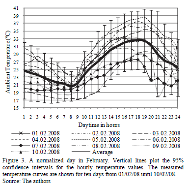
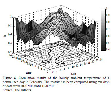
A total of 91 normalized daily ambient temperature profiles were determined by using the routine presented in section 3.2., Step 3. For this purpose, the time period covered by database 1, i.e., from 20/01/08 to 31/07/10, was considered. Each one of these 91 normalized days is representative of a day in a month of the year; i.e., there are 7 normalized days representing a day in January, 9 normalized days representing a day in February, 9 for March, …, etc. For example, a normalized ambient temperature for a day in February, obtained from the population of 10 days from 01/02/08 to 10/02/08, is shown in Fig. 3. The vertical lines indicate the probabilistic distribution of the normalized hourly temperature. Moreover, the mesh that represents the correlation matrix for that normalized day is plotted in Fig. 4. A strong correlation between the hourly ambient temperatures, especially for those that are adjacent, is observed.

4) Step 4. Ambient temperatures were then determined for the 01/01/01 - 19/01/08 period. The minimum and maximum temperature values of the 91 normalized days were employed as features of typical days. From these features and from the daily minimum and maximum temperatures that are shown in database 2, the Euclidean distances were computed by using . In this way, one of the 91 normalized days was assigned to each day between 01/01/01 and 19/01/08. Subsequently, the corresponding monthly average temperatures were calculated for this period. The assigned normalized days were scaled by the ratio of the calculated monthly average temperatures over the real monthly average temperature given in database 3. As such, the monthly average temperatures, including assigned normalized days from the 01/01/01 - 19/01/08 period coincide with the real monthly average values that are given for the same period.

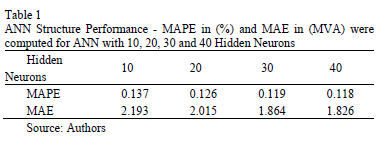
5) Step 5. The lacking load values have to be estimated for the 15/02/94 - 19/01/08 period. ANN structures, such as those shown in Fig. 1, with 10, 20, 30 and 40 hidden neurons were tested. The performance of these structures was verified by two measures: i) the mean absolute percentage error (MAPE), and ii) the mean absolute error (MAE).

where n is the total number of load values between 20/01/08 - 31/07/10, LM,i and LF,i are the measured and forecasted hourly load values, in MVA, respectively. The performance values for each ANN are given in Table 1.

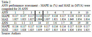
By increasing the number of hidden neurons, the performance of the ANN improves. However, there is only a small improvement for more than 30 hidden neurons. Therefore, a structure of 40 hidden neurons was implemented. Moreover, when training an ANN, the initial weights and biases of the network are usually randomly generated taking values between -1 and 1. This initialization has the ability to produce an improved network. Therefore, twenty two-layer feed-forward networks with 40 hidden neurons were created and trained for the 20/01/08 - 31/07/10 period. With the real load values and those estimated through the ANN, the performance of these 20 ANNs was verified again by means of MAPE and MAE. The performance values for each one of these 20 ANNs are given in Table 2.

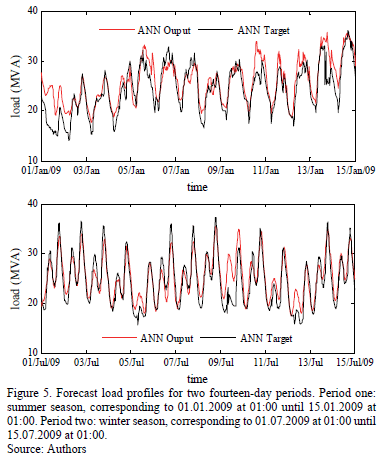
Network 4, which showed the best performance, was chosen for its back-in-time estimation of load. Diagrams in Fig. 5 show the forecast loads for two different fourteen-day periods. It can be observed from the graphical results that the forecast load follows the real measured values closely.

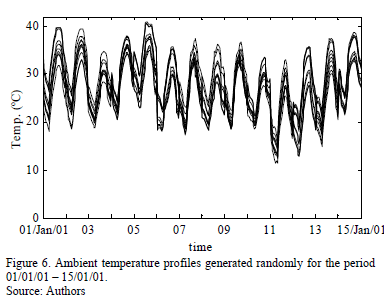
6) Step 6. Probable ambient temperature profiles were created by using MCS. A thousand ambient temperature profiles, L=1000, each containing 123168 temperature values included in the period 15/02/94 - 19/01/08, were generated by multivariate normal random numbers. These numbers were computed from the hourly normal distributions characterized by the mean hourly ambient temperature, , the corresponding standard deviation, , and the daily covariance matrix, S_d that were obtained in steps 3 and 4.

Once the probable ambient temperature profiles were obtained, they were constrained to fit the reported information given in database 3, e.g., 10 randomly generated ambient temperature profiles for the first 15 days of January of 2001 are shown in Fig. 6.

The selected ANN network was then used to estimate 1000 of the transformer's probable load profiles. Each hourly load profile was estimated from a corresponding probable temperature curve and the input data from database 4.

7) Step 7. The HST model presented in section 2.2 was adjusted for the unit characteristics of the case study. Moreover, to deal with the changes in the cooling modes, ONAN/ONAF, it was necessary to model the behavior of the temperature monitor that commands the fans. This type of device uses the following approach to estimate the control HST:

where, H and y are set values which depend on the transformer characteristics, in fact, in this case study, H=1.3 and y=1.6. It must be noted that the control HST (q_HS,c) computed from is an approximation, the only purpose of which is to command the fans. In fact, fans are turned-on when q_HS,c is higher than 85ºC, and turned-off when q_HS,c becomes lower than 75ºC so as to avoid repetitive on-off fan operations.

In the algorithm that was implemented, when both q_TO, computed from , and K (which depends on the load) yield q_HS,c values higher than 85ºC; when the temperature is increasing, or lower than 75ºC; or when the temperature is decreasing, then the empiric constants n and m in eq. - change and assume their respective values in agreement with the activated cooling mode.

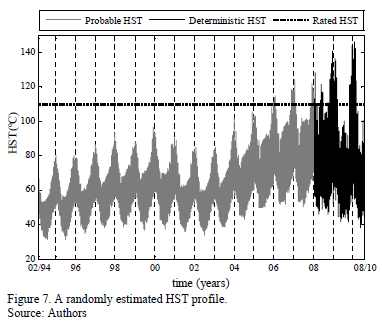
The HST calculation was divided into two parts. The first part is the deterministic HST calculation based on the load profile data covering the period from 20/01/08 to 31/07/10.

The second part is the probabilistic HST calculation that was made for all 1000 estimated load and ambient temperature profiles determined for the 02/15/94 to 19/01/08 period. Therefore, 1000 HST curves were computed. One of these HST-curves is shown in Fig. 7.

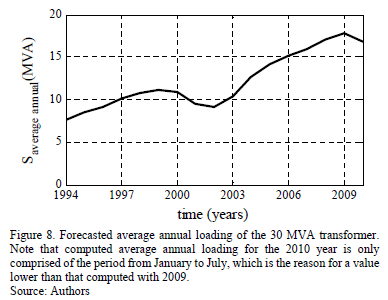
Moreover, Fig. 8 presents a diagram showing the average annual loading. This data shows the loading trend of the 30 MVA transformer. A fact it is worthwhile pointing out is the sudden decrease in the demand that timely coincided with the 2001 political and financial crisis in Argentina; this is also reflected in the forecasted load.

8) Step 8. After pre-processing the load profile data, estimating the ambient temperature and the load, and subsequently determining the 1000 probable HST profiles for the 15/02/94 - 31/07/10 period, the functional age of paper was determined. The first component functional age is deterministic, and corresponds with the accumulated age during the period 20/01/08 to 31/07/10. This was computed by using, , the accelerated aging factor for thermally-upgraded paper, and, , the functional age, AF, of insulating paper. The resulting functional age for this period was 8415.5 hours.

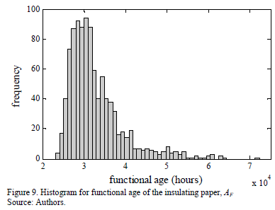
The second component of AF is probabilistic, and it was estimated for all the 1000 probable HST profiles, also by means of and . Therefore, L=1000 probable values for the AF of the insulating paper were estimated for the 15/02/94 to 19/01/08 period. The total AF of the insulating paper was computed by adding both the deterministic and the probabilistic components. Fig. 9 shows the distribution of the total AF in a histogram of 50 bins.

9) Step 9. It was observed from the results that 90% of computed AF are less than 41376 hours, and 95% (950) of the simulations yield to AF values lower than 47739 hours.

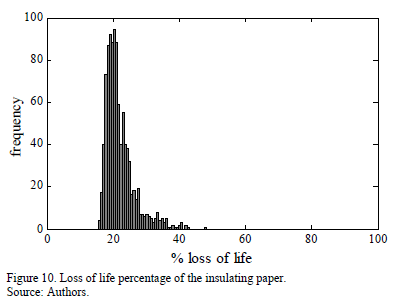
Finally, the los-of-insulation life percentage, due to thermal aging, was computed by using , and the DP=200 end of life criterion. As such we obtained the histogram shown in Fig. 10, in which it can be observed that the studied power transformer's insulating paper is still in good condition, from a thermal aging point of view. In fact, from the histogram, it can be seen that the bin centered at 21.4% loss of life value reports the highest frequency of occurrence , i.e. it represents the mode.

 

5. Validation

In this section the performance of the proposed methodology is assessed.

5.1. Probabilistic method assessment

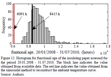
The result obtained in section 4.2, step 8, (A_F = 8415.5 hours for the 20/01/08 to 31/07/10 period), i.e. the period for which hourly ambient temperature and load profiles are available, is compared with those obtained by assuming that data was not recorded. For this purpose, historical daily minimum and maximum temperatures, obtained from 91 normalized daily ambient temperature profiles and trained ANN were used to assess the probable A_F by means of MSC. The most frequent bin (in effect, that containing 91 simulations) is the one centered in 8680 h, with edge values of 8580 h and 8790 h. Additionally, 950 simulations (95%) yield lower values than 11119 h.

5.2. Assessment of ambient temperature reconstruction methods, founded on sinusoidal functions of time

References [22] and [23] present deterministic methods to produce hourly temperature data by assuming that yearly temperature amplitudes and hourly temperatures follow sinusoidal functions of time. To assess the performance of such proposals, again, a comparison of the results obtained from the period 20/01/08 to 31/07/10 was undertaken.

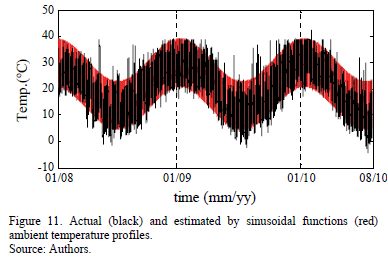
In Fig. 11, actual and estimated by the sinusoidal functions of time ambient temperature profiles are plotted. From the estimated profile, the A_F calculation is performed, obtaining a result of 6091 h.

This result shows that A_F is underestimated when the sinusoidal functions of time are employed to reconstruct the ambient temperature. A possible explanation for this result is that hot days are omitted for periods falling out of the hottest month; this can be observed in Fig. 11.

5.3. Discussion

The results obtained from test in sections 5.1 and 5.2 are shown in Fig. 12. The deterministic result obtained in 4.2, and the central value of the most frequent bin obtained in 4.1 are compared with the reference of 8415.5 h in Table 3.

These results show that the probabilistic method proposed for the reconstruction of ambient temperature curve could lead to results that do not underestimate the functional age of the insulating paper. Moreover, the results also highlight that the proposed method is able to model the uncertainty involved in the problem that is the motivation for this paper.

To conclude this discussion, there is a lot of research that needs to be done in order to achieve a higher degree of accuracy in the predictions about the transformer condition. It is widely recognized that in this problem there are several sources of uncertainty. For instance, there is uncertainty in the measurement and posterior diagnostic model of frequency response analysis when looking for faults in core and coils [24-26]. The situation is the same for DGA when oil is analyzed (in fact, there are several methods to infer incipient faults in the transformer through DGA, but none of these can be considered as the best one). Furan analysis to infer the DP, is affected by changes in oil, uncertainty about the mass of insulating paper, the type of paper, etc.

In this context, it is expected that models to assess the loading history of a transformer may also be affected by uncertainty. There is uncertainty affecting ; i.e., about the constant B=15000. There have been different values reported in [5]. Moreover, as stated in section 2.1, the reference value for end-of-insulation life and the Arrhenius plot are also affected by the three insulating paper aging mechanisms, hydrolysis, pyrolysis and oxidation.

Finally, there is also uncertainty when one attempts to reconstruct historical load and ambient temperature profiles (especially in the adopted forecasted models, which undoubtedly can be improved, e.g., by testing other ANN structures, or employing hybrid methods as ARIMA-ANN). However, it is noted that one of the major contributions reported in this paper is related to the capability of the proposed method in modeling uncertainty. Most of the standard methods are deterministic. Therefore, these do not recognize the uncertain nature of the analyzed problem.

 

6. Conclusions

This paper introduces a methodology to estimate missing load data to be used in order to determine the functional age of power transformers' insulating paper. The methodology is founded on the statistical analysis of local ambient temperatures, and on ANNs and MCS to estimate probable historical HST profiles. Subsequently, through the thermal aging principles of insulating paper, it is possible to assess the functional age and loss-of-insulation life percentage due to thermal effects.

Later on in the research, a case study for a 30 MVA rated transformer with its corresponding database was presented. Based on this database and on long term temperature measurements from an external weather station, through MCS, 1000 probable ambient temperature curves were generated for the whole operational period of the unit. Then, using an ANN 1000, probable load profiles were obtained. With these results, a corresponding number of HST profiles were then gathered.

Test results were processed to estimate the frequency of the occurrence of the studied transformer's functional age. The results obtained show that the insulating paper from the unit under investigation is still in good condition, in terms of a thermal aging point of view and from its loading history analysis. Moreover, it was shown that calculation of functional age is also useful to estimate the loss of life percentage due to thermal aging. The presented methodology will contribute to the transformer condition monitoring as a cheap, comparably fast and easily accessible tool, even for load profiles that do not contain the entire load and ambient temperature data for the whole period of unit operation.

Further research on this issue must be conducted in order for several other important aspects to be considered. These include the following in particular: to include in the model influence of moisture on the aging speed, to improve the forecasting accuracy by testing hybrid methods as ARIMA-ANN, and to assess both the functional age and the loss-of-insulation life percentage in forecasted future load scenarios. Finally, the proposed method is an applicable tool for a major project research that is searching for the determination of a transformer risk index.

 

References

[1] Li, W., Risk assessment of power systems, models, methods and applications. IEEE Press Series on Power Engineering, 2005.         [ Links ]

[2] Romero, A.A., Mombello, E.E. and Rattá, G., An overview on power transformer management: Individual assets and fleets, Transmission and Distribution Latin America Conference and Exposition (T&D-LA), Sixth IEEE/PES, pp. 1-7, 2012. DOI: 10.1109/TDC-LA.2012.6319081        [ Links ]

[3] CIGRE Brochure 323. Aging of cellulose in mineral-oil insulated transformers. Taskforce D1.01.10, Ed. 2007.         [ Links ]

[4] Lelekakis, N., Wenyu, G., Martin, D., Wijaya, J. and Susa, D., A field study of aging in paper-oil insulation systems, IEEE Electrical Insulation Magazine, 28(1), pp. 12-19, 2012. DOI: 10.1109/MEI.2012.6130527        [ Links ]

[5] IEEE Guide for loading mineral-oil-immersed transformers and step-voltage regulators. IEEE Standard C57.91, 2011.         [ Links ]

[6] IEC Power Transformers, Part 7: Loading guide for oil-immersed power transformers. IEC 60076-7, 2005.         [ Links ]

[7] Susa, D. and Nordman, H., A simple model for calculating transformer hot-spot temperature, IEEE Transactions on Power Delivery, 24(3), pp. 1257-1265, 2009. DOI: 10.1109/TPWRD.2009.2022670        [ Links ]

[8] Susa, D. and Lehtonen, M., Dynamic thermal modeling of power transformers: further Development-part I, IEEE Transactions on Power Delivery, 21(4), pp. 1961-1970, 2006. DOI: 10.1109/TPWRD.2005.864069        [ Links ]

[9] Susa, D. and Lehtonen, M., Dynamic thermal modeling of power transformers: further Development-part II, IEEE Transactions on Power Delivery, 21(4), pp. 1971-1980, 2006. DOI: 10.1109/TPWRD.2005.864068        [ Links ]

[10] Lundgaard, L.E., Hansen, W., Linhjell, D. and Painter, T.J., Aging of oil-impregnated paper in power transformers, IEEE Transactions on Power Delivery, 19(1), pp. 230-239, 2004. DOI: 10.1109/TPWRD.2003.820175        [ Links ]

[11] CIGRE, Moisture equilibrium and moisture migration within transformer insulation systems, Vol. A2.30, Ed, 2008        [ Links ]

[12] Du, Y., Zahn, M., Lesieutre, B.C., Mamishev, A.V. and Lindgren, S.R., Moisture equilibrium in transformer paper-oil systems, IEEE Electrical Insulation Magazine, 15(1), pp. 11-20, 1999. DOI: 10.1109/57.744585        [ Links ]

[13] Fofana, I., Borsi, H. and Gockenbach, E., Fundamental investigations on some transformer liquids under various outdoor conditions, IEEE Transactions on Dielectrics and Electrical Insulation, 8(6), pp. 1040-1047, 2001. DOI: 10.1109/94.971463        [ Links ]

[14] Oommen, T. and Prevost, T., Cellulose insulation in oil-filled power transformers: Part II - Maintaining insulation integrity and life, IEEE Electrical Insulation Magazine, 22(2), pp. 5-14, 2006. http://dx.doi.org/10.1109/MEI.2006.1618996        [ Links ]

[15] Lobo-Ribeiro, A.B., Eira, N.F., Sousa, J.M., Guerreiro, P.T. and Salcedo, J.R., Multipoint fiber-optic hot-spot sensing network integrated into high power transformer for continuous monitoring, IEEE Sensors Journal, 8(7), pp. 1264-1267, 2008. DOI: 10.1109/JSEN.2008.926926        [ Links ]

[16] Jauregui-Rivera, L. and Tylavsky, D., Acceptability of four transformer top-oil thermal models - Part II: Comparing metrics, IEEE Transactions on Power Delivery, 23(2), pp. 868-872, 2008. DOI: 10.1109/TPWRD.2007.905576        [ Links ]

[17] Peña., D., Análisis de datos multivariantes, Mc Graw Hill, 2002.         [ Links ]

[18] Zhang, G.P., Time series forecasting using a hybrid ARIMA and neural network model, Neurocomputing, 50, pp.159-175, 2003        [ Links ]

[19] El-Desouky, A.A. and Elkateb, M.M., Hybrid adaptive techniques for electric-load forecast using ANN and ARIMA, IEE Proceedings Generation, Transmission and Distribution, 147(4), pp.213-217, 2000. DOI: 10.1049/ip-gtd:20000521        [ Links ]

[20] Feinberg, E. and Genethliou, D., Applied mathematics for restructured electric power systems - Chapter 12: Load Forecasting. Springer, Hamburg, 2005, pp. 269-285.         [ Links ]

[21] Hornik, K., Stinchcombe, M. and White, H., Multilayer feedforward networks are universal approximators, Neural Networks, 2(5), pp. 359-366, 1989.         [ Links ]

[22] IEC, Loading guide for oil-immersed power transformers, IEC 60354, Second edition, 1991.         [ Links ]

[23] Gelegenis, J.J., Estimation of hourly temperature data from their monthly average values: case study of Greece, Renewable Energy, 18(1), pp. 49-60, 1999.         [ Links ]

[24] Gómez-Luna, E., Fernando-Navas, D., Aponte-Mayor, G. and Betancourt-Buitrago, L.A., Literature review methodology for scientific and information management, through its structuring and systematization, DYNA, 81(184), pp. 158-163., 2014 DOI: 10.15446/dyna.v81n184.37066        [ Links ]

[25] Gomez-Luna, E., Duarte, C., Aponte, G., Guerra, J.P. and Goossen, K.W., Experiences with non-intrusive monitoring of distribution transformers based on the on-line frequency response, Ingeniería e Investigación, 35(1), pp. 55-59, 2015. DOI: 10.15446/ing.investig.v35n1.47363        [ Links ]

[26] Gomez-Luna, E., Aponte, G., Herrera, W. and Pleite, J., Experimentally obtaining on-line FRA in transformers by injecting controlled pulses, Ingenieria e Investigacion, 33(1), pp. 43-45, 2013.         [ Links ]

 

A.A. Romero-Quete, was born in Colombia in 1978. He received a degree in Electrical Engineering in 2002, from the Universidad Nacional de Colombia, and his Ph.D. from the Universidad Nacional de San Juan (UNSJ) in 2009. He is currently a researcher at the Consejo Nacional de Investigaciones Científicas y Técnicas, CONICET, at the IEE UNSJ-CONICET. His research interests are: asset management, power quality, and high voltage test techniques. ORCID: 0000-0002-6530-852X

E.E. Mombello, was born in Buenos Aires, Argentina, in 1957. He received a B.S. in electrical engineering and a Ph.D. in electrical engineering in 1982 and 1998, respectively. He has worked for CONICET, at the Instituto de Energia Electrica of the University of San Juan (IEE-UNSJ), Argentina, as a lecturer and researcher since 1982. His main fields of interest are design, modeling and diagnostics of power transformers, transformer life management, electromagnetic transients in electric machines and networks, modeling of equipment, low frequency electromagnetic fields. ORCID: 0000-0003-0425-596X

G. Rattá, was born in Italy in 1950. He received his degree in Electromechanical Engineering from the Universidad Nacional de Cuyo-Argentina in 1974. Since 1997 he has been director of the IEE-UNSJ, Argentina. Prof. Rattá is currently an Assistant Professor in the UNSJ. His research interests include transient behavior of power system components and power quality. Email: ratta@iee.unsj.edu.ar. ORCID: 0000-0003-3663-6310