


 English (pdf)
 Article in xml format
 Article references
 Send this article by e-mail
 Cited by SciELO
  Cited by Google
  Similars in
SciELO
Similars in
SciELO  Similars in Google
 Permalink
1. Introduction
A wetland is an ecosystem in which the permanent or temporal excess of water and the resultant lack of oxygen are the main factors determining soil formation and flora and fauna communities [1]. The range of services provided by wetlands varies depending on the location of the watershed they are in (inland, riverline, or coastal) and the size of the wetland; in any case, wetlands are generally assumed to play important ecosystem functions such as providing habitat and shelter for wildlife species, erosion control, sediment and nutrient removal, and regulation of stream discharge. Additionally, wetlands are becoming increasingly important in flood control owing to expected increases in extreme rainfall as a result of climate change [2,3]. Recent developments to define wetland functions have emphasized their spatial variation, including geomorphology [4], as well as their dynamics due to climate variation [5].
The importance of wetlands and their spatial extension across boundaries have been recognized by policy makers and the research community [6], especially when considering that during the 20th century they were drained or degraded [7]. Three large international commitments have been proposed due to the transnational nature of wetlands: the Rio declaration, the Langkawi declaration and the Ramsar convention. However, decision-making regarding wetland management is difficult because there are frequently opposing objectives between conservation and economic development [8], unclear wetland delimitation and inadequate planning. Additionally, in tropical developing countries land tenure regimes are complex, laws are often contradictory and land rights unclear [9].
Defining spatial boundaries for ecological ecosystems is an important step towards management [10]. Wetlands are commonly identified and delineated based on the coexistence of three factors occurring within the same spatial domain: hydromorphic soils, hydrophytic vegetation and wetland hydrology. However, implementing this definition is problematic because of the fuzzy nature of the interphase between aquatic and terrestrial ecosystems, and because the definition assumes that all factors are occurring at the same time. In fact, evidence of a single factor may be sufficient to determine whether a wetland exists. For instance, recurrent flooding in an area where hydrophytic vegetation has been removed is indicative of the presence of a wetland. Natural vegetation removal and modification of surface hydrology using levees, channels and pumps are additional challenges to determine wetland extent. The impact of development on wetlands was classified by Nelson and Weller [11] as a function of the extent, permanence and cost of the remedy.
Despite the importance of neotropical wetlands in terms of biodiversity conservation [12,13] and flood control [3], information regarding wetlands distribution in northern South America is limited [14] and data on functions, processes and values are scarce [15]. Therefore, this study was conducted to identify areas with wetland potential taking into account hydromorphic soils, hydrophytic vegetation, phreatic fluctuations and inundated areas. Special attention was paid to characterization of water depth through measurement of piezometric levels, as well as characterization of inundated areas by remote sensing [16-18]. The results are combined using a binary method, flexible enough to allow for different criteria based on the current wetland condition. The goals of this study are: i) to model environmental variables and design an objective method to determine potential areas of wetlands; ii) to characterize changes in surface hydrology due to infrastructure;
iii) to determine implications of further agricultural development on natural resources.
2. Study site
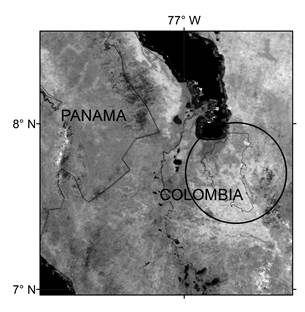
The floodplain of the Leon River takes up an area of 1029 km2 (anaerobic soil conditions, mean slope = 4%), located in the northern hemisphere of the neotropics. The river flows to the Caribbean Sea between the Atrato River and the Abibe mountain range (Fig. 1). These rivers are characterized by high sediment load [19] and the quality of groundwater, which is affected by land use activities such as mining, large scale agriculture (banana and plantain) and cattle grazing [20]. In general, these hydromorphic soils act as sinks of surface runoff from urban and agricultural activities where best management practices (BMP) are required to mitigate adverse effects on aquatic systems [21]. In addition, two large development projects are expected in the near future: a marine cargo port at the León River outlet and the Pan-American Highway to communicate South America and Central America.
The hydrological regime of this region is associated with the movement of Intertropical Convergence Zones (ITCZ) [22] with unimodal behavior, resulting in a dry season starting in January with the lowest stream discharge around March, and a wet season during the rest of year, peaking in June, July and August. The maximum daily precipitation measured by IDEAM at rain gauge stations is particularly high (216 mm/day), with an annual precipitation range between 2300-4200 mm and an average temperature of 28°C; therefore, the region is classified as a humid tropical forest.
3. Materials and methods
Five variables related to biophysical characteristics of wetland ecosystems were selected from expert knowledge: hydromorphic soils, hydrophytic vegetation, surface hydrology, piezometric ground water levels and a wetness index. A per pixel binary system was used to determine wetland presence or absence for each variable, then the combination of variables resulted in different wetland potential. Wetland potential is required to define detailed objectives of environmental management. The maximum level of detail available was used since the ability to define boundaries is closely related to the spatial resolution of the data [23]. Remote sensing was used to delineate hydrophytic vegetation and inundated areas, whereas GIS was used to calculate a wetness index and a groundwater model. GIS and remote sensing techniques are considered reliable, verifiable and efficient to monitor wetland ecosystems [24-27]. Given the limitations of remote sensing to determine piezometric levels and soil types, these variables were obtained from field measurements of piezometric levels and maps from the National Geographic Institute “Agustín Codazzi”. Variables were classified in two wetland classes: swamps and marshes.
Source: The authors.
Figure 1 Wetlands associated with the Atrato River, León River floodplain located near the boundaries of Panamá and Colombia, South America. The background is a MODIS satellite image with 250 m spatial resolution.
3.1. Surface hydrology
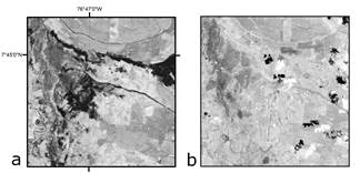
Satellite images were used to identify the marsh class, commonly occurring along rivers, ponds and lakes [28]. All satellite images of the Landsat program with world reference system (WRS) path 10 row 55 were evaluated. Satellite images have been found useful in tropical areas where fieldwork is not feasible owing to the harsh physical conditions [29]. Spatial distribution of inundated areas was determined making use of the temporal detection method of paired images [30, 31]: this method requires images of the same site, in this case after and before a flood in order to avoid confusion of flooded areas with other surfaces of similar reflectance as dark soils or shadows (Fig. 2). Visual interpretation of satellite imagery was preferred over fieldwork to delineate inundated areas because of the ephemeral nature of floods. The error here is related to the pixel size of 30 m of a Landsat image, commonly associated to a 1:100.000 map scale.
Landsat optical remote sensing satellites TM4, TM5 and ETM7 include sensors on the visible, Near Infrared and Small Wave Infrared (SWIR) wavelengths. Wavelengths at the SWIR are important due to their high sensitivity to water content [32]. The best image found showing inundated areas was the ETM+ taken on August 27, 2011 during the positive phase of El Niño [3], which is characterized by flooding in Colombia, Brazil, Argentina and Venezuela.
Source: The authors.
Figure. 2 Paired method image interpretation as ground truth of inundated areas. Dark tones in (a) are inundated areas.
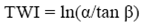
Another approach to determine the extent of inundated areas was the topographic wetness index (TWI) eq. 1. Different topographic indexes area available to predict wetland distribution [33], based on the direction and accumulation of water flow derived from a digital elevation model (DEM). The TWI was calculated as the ratio of the slope (degrees) to the upslope of the contributing area.
 (1)
(1)
There are several methods used to compute this index depending on the algebraic order of the ratio and the method employed to calculate the upslope contributing area [34]. Here, the contributing area was calculated using the single direction D8 flow model [35], which includes the area of each raster cell plus the contribution of upslope neighbor cells. Because the contributing area is always higher than zero it was used as the denominator of the ratio. The SRTM (shuttle radar topography mission) with 30 m spatial resolution was selected as the DEM input for the TWI.
Two additional aspects regarding human-induced activities on surface hydrology were also considered: river diversion and non-natural levees. A total of 64 cross sections (sections normal to the direction of river flow) were located along an existing map of artificial levees; each cross section was georeferenced with a submetrical GPS. A total station was used to survey the geometry of each cross section, field work was carried out during the dry season in order to avoid flooding conditions.
3.2. Hydromorphic soils
Hydromorphic soils were extracted from the official soils map of the Geographic Institute “Agustín Codazzi” with a minimum mapping unit of 5 ha. Two soil studies were available for this area, a semi-detailed study of soils with potential for agriculture in the Urabá region (1:25,000) [36], and a general study of soils for the state of Antioquia (1:100,000) [37]. The profile description of each Soil Map Unit (SMU), including information about topography, humidity regime, texture and color, was used to categorize soils into two different soil moisture regimes [38]. Specifically, hydromorphic soils were characterized as Aquic, in which the phreatic level is close to or over the soil surface for long periods (gleysols) with reducing conditions, or Udic, where soil is not dry for more than 90 cumulative days during a year. Soils along the coast of the Caribbean Sea are covered or saturated by tidal freshwater, seagrass meadows and mangroves.
3.3. Hydrophytic vegetation
A series of polygon maps derived from satellite images were used to characterize the temporal and spatial distribution of vegetation. Satellite images are important in the context of wetland studies since they provide periodical observations, information of wetland surroundings and images that are easily integrated into a Geographical Information System [39]. A digital map was available for 2007 based on the visual interpretation of SPOT and ASTER images, then a set of RapidEye images of 2012 were used to update the 2007 version. An error matrix was calculated for assessing the accuracy of the vegetation map [40]. Reference data to validate this variable were collected during ground visits (along river and roads) and from Ortho-rectified color aerial photographs with spatial resolution of 0.5 m; photographs were used in areas not covered during ground visits. A random sample of 300 sites was used to calculate error matrix, kappa coefficient and overall accuracy.
All polygons defined as grasslands or natural forests were visited by boat along the León River in order to identify hydrophytic species. Polygons in which hydrophytic species constituted the dominant vegetation were classified as swamps (Prioria copaifera, Raphia taedigera, Montricharida arborescens, Camnosperma panamensis, Euterpe oleracea, Thypha dominguensis, Heliconia spp. and Paspalum fasciculatum). Mangroves are dominant along these coasts, the spatial distribution of these species is available from the inventory of Giri et al. [41]. From an agricultural perspective, two introduced species are of importance owing to their spread in the study area, Brachiaria arrecta, which was imported from Africa and adapted to grow on seasonally inundated areas, and banana and plantain Musa spp. from Asia. Banana plantations are well distributed throughout wet tropical regions, including Central America, Colombia and Ecuador.
3.4. Piezometric model
Temporal variation of phreatic surfaces was used to identify wetlands since these variations can act as boundaries that depict inundated areas. In this case, the vertical variations of the aquifer were determined from piezometric levels at 41 monitoring wells during 29 different campaigns. Well locations were determined with a sub-metric GPS and water depth was measured with a bipolar electric probe calculating every centimeter; this network of wells was used to generate a model of piezometric levels with spatial interpolation [42,43]. The kriging interpolation method was used to generate a model of piezometric levels (SPL) for each campaign resulting in 29 raster layers; cross validation was applied in order to measure the predictive performance of this model. When a piezometric level was found to be higher than or equal to the digital elevation model (DEM) from the
Shuttle Radar Topography Mission (SRTM) the area was marked as inundated. A summary layer was created from all areas that were inundated on at least one occasion (PL≥DEM).
3.5. Binary decision method
To summarize the previous five variables in terms of wetland potential, a Boolean logic was applied. The binary decision method allows definition of mandatory variables, summation of variables, or definition of many combinations as 2n, where n is the number of variables. Each variable was treated as a raster layer with a pixel size of 30 m and each pixel of the raster was reclassified into a binary condition of (0) or (1) based on the expert decision. Specifically, 0=false where the spatial extent (area) of the variable had no evidence of a wetland and 1=true where the expert had evidence of a wetland. The variables were then overlaid to create a data cube, where the x,y axes are the pixel spatial distribution, and the z axis is the binary condition of each variable. The binary approach allows for a number of binary combinations as a function of the number of variables, in this case 25=32. The binary approach allows to define a set of conditional rules on the z axis and define the potential area for wetlands. Four logical rules were used, given priority to those variables with field validation, i.e., hydrophytic vegetation and inundated areas (identified by the pair satellite images method or by the piezometric model). Any pixel with evidence of hydrophytic vegetation or evidence of inundation was classified as wetland, while the other two variables, soils and TWI were defined as potential area for wetland only when coexisting. The four logical rules used to define the potential of “wetland pixels” were:
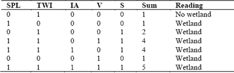
Table 1 Example of possible variable combinations using the logic rules. S…Hydromorphic soils, V…Vegetation, SPL…Summary of piezometric levels (PL≥DEM), IA… Inundated areas observed from satellite image interpretation, TWI…Topographic wetness index.
Source: The authors
Evidence of hydrophytic vegetation from the vegetation map.
Detected inundated areas following the interpretation of paired satellite images.
Inundated areas based on the piezometric model.
Two or more variables occurring at the same location (sum ≥ 2).
Hydrophytic vegetation is a clear indicator of wetland presence, but it has partially been removed through decades of land use change to crops or grasslands. For this reason, the piezometric model, TWI and Soils were considered relevant wetland indicators. TWI and hydromorphic soils were included as wetland candidates only when coexisting at the same location through the logic rule (sum≥ 2), i.e., two variables indicating wetland presence. Table 1 shows an example of seven binary combinations and their reading in terms of wetland presence. For instance, (00000) represents no wetland evidence while (01001) or (11011) indicates that no hydrophytic vegetation remains but there is evidence of wetlands from other variables.
4. Results
4.1. Surface hydrology
Although use of satellite images provides a direct method for determining inundated areas, the use of optical data is a challenge, given the high cloud content during the wet season and the absence of inundated areas during the dry season, when the sky tends to be clear [44]. Another technical difficulty associated with optical data was the interpretation of inundated areas below banana crops and swamps with dense canopy cover. The total inundated areas (147 km2) identified by the Landsat satellite image of August 2011 were marshes along the León River and its tributaries; despite tidal changes at the study area being minor, the effect on the last 5 km of the river was evident during field work . The rest of the inundated areas are non-tidal marshes. It is important to note that a single satellite image only represents the inundated spatial distribution of that particular instant; accordingly, the extent of inundated areas is likely larger since August, the observed month, is not the wettest one.
High per pixel values of TWI are related to large contributing areas and lower slopes, i.e., areas where surface runoff is likely to concentrate. The threshold to define the extent of TWI wetland pixels was defined by expert knowledge and regional topography. The area of candidate wetland pixels for this variable totals 218 km2, the quality of this result is a function of the level of detail and the relative elevation difference among pixels of the DEM. The SRTM input data for the TWI model was validated using GNSS RTK sub-metric measurements along the Leon River. Despite the pattern of the DEM depicting the general slope of the river flowing towards the sea, large elevations differences were found along the estuary, given the height of the forest along the borders, the spatial resolution of the DEM of 30 m (Fig. 3) and the difference between orthometric and WGS84 models.
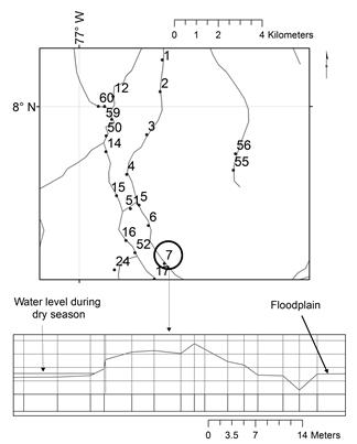
Surface hydrology has been modified by the construction of artificial levees and diversion channels. Levees characterized during field work are distributed parallel to the main channel and tributaries (Fig. 4). Levees failure was observed along the main channel since the alluvial materials used to build them are highly erodible and these structures are commonly found on unstable soils. This fact is aggravated in those areas where water is conveyed above or at floodplain level. Another concern is the long term viability of this practice, since it prevents lateral flow of sediments from reaching the floodplain. Therefore, sediments are deposited only within the river bed, reducing its cross section area and forcing the construction of ever higher and wider levees to prevent overflowing. This feedback potentially increases the hazard of flooding in areas surrounding levees and downstream. Unfortunately, the TWI model does not take into account levees, given the coarse resolution of the SRTM data [45]. The average height of levees is 2.3 m, minimum 0.6 m and maximum 4.6 m (n=46). Two diversion points were also identified using satellite imagery: the diversion from the Leon River to the Tumaradó Lake and the diversion from the Leon River to the Suriquí River, both located inside the areas of high flow accumulation identified by TWI.
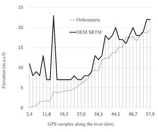
Source: The authors.
Figure 3 Differences in elevation from the estuary to the upper boundaries of the wetland along the river line.
Levees were constructed along the main channel and tributaries to restrict lateral flow with two different objectives: on the one hand, to protect banana crops and cattle from river overflow, and on the other hand, to promote deposition by trapping sediments as a mechanism for land preparation. However, restrictions to river discharge may cause unexpected results. For instance, flooding increase at lower reaches is likely to occur as flood water storage is no longer provided upstream along the river floodplain for extreme events.
4.2. Hydromorphic soils
The surface area of Udic soils (76%) and Aquic soils (23%) dominated the floodplain with a minor presence of soil under aerobic conditions (1%). Overall, 77% of these soils are covered by cattle grazing and banana crops with complex drainage systems; accordingly, only Aquic soils were considered wetland and Udic soils excluded because of the severe modifications generated by establishment of agriculture. With these findings and based on the official soil´s map, the area of wetland pixels is 234 km2 (Fig. 5).
4.3. Hydrophytic vegetation
Hydrophytic vegetation is mainly located in the north, near the estuary, with a total area of 167 km2 (Fig. 5). Validating the classification of remote sensing is straightforward when using the error matrix since reference information is available in the field (Table 2). The 2012 version of the vegetation map was based on a RapidEye image with 5 m spatial resolution and a minimum mapping unit of 0.5 ha meeting the standards of a 1:25000 scale. The overall accuracy of the vegetation map was 80.66% with a Kappa coefficient of 0.76.
4.4. Piezometric model
The wetland area determined by the piezometric model (SPL) was 305 km2 (Fig 5); this area was validated using well measurements. The Kriging model was defined by the following parameters: A Range value of 45,512.25086939145, a Partial Sill value of 1.42967383653 and Nugget value of 0. Results of the interpolated piezometric levels were tested using cross-validation. This validation method calculates statistics which provide an unbiased and accurate prediction of parameter values. The main error was 0.08 m with an average standard error of 3.89 m. These values are acceptable when compared to the range of the height values (> 20 m) of the study area.
4.5. Wetland potential based on a binary decision method
Different arrangements of the binary decision method provide extreme differences in the extent of the potential wetland area. The area covered with one variable or more meeting the wetland conditions (binary sum ≥ 1) is 536 km2, while the area with all the variables occurring at the same pixel (binary sum = 5) is only 0.6 km2. Out of the 32 possible binary combinations, 28 defined wetland condition because of rules 1, 2 or 3. Only one binary combination defined wetland condition because of rule number 4 (01001) (Fig. 6).
Table 2 Accuracy assessment of vegetation based on the matrix error. Reference data

Source: The authors
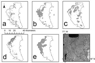
Source: The authors.
Figure 5 Binary representations of variables associated with wetland conditions. (a) Inundated areas, (b) Topographic wetness index, (c) Hydromorphic soils, (d) Hydrophytic vegetation, (e) Piezometric model, (f) Leon River stream network and floodplain with a Landsat image ETM+.
Approximately one third of the floodplain (393 km2) was classified as wetland when considering the four logical rules. The most important binary combinations in terms of wetland area were (10000), (11000) and (00100) indicating the large extent of the piezometric model and the inundated areas. Combinations (11011) and (10011) are also important wetland candidates because of the extent, 18 km2 and 29 km2 respectively, and the amount of variables meeting the wetland condition. Logical rule number 4 classified only 3% of the area as wetland. These 11 km2 of agreement between TWI and hydromorphic soils (01001) where hydromorphic vegetation was removed, are important in terms of natural resource management because of the large potential to recover pre-disturbance conditions. The selection of wetland pixels using the logical rules allows the identification of a large area in the northwest portion of the study area surrounded by scattered clusters along the floodplain. Three binary combinations resulted in no wetland potential because there was no evidence from biophysical variables (00000) with 493 km2 or only evidence of hydromorphic soils (00001) with 118 km2 or TWI (01000) with 24 km2. Large extension of hydromorphic soils are distributed to the east of the floodplain where no other variables reaffirm the wetland potential (Fig. 5).
There are several implications on conservation and agriculture expansion when defining wetland potential from Fig. 6. From the 324 km2 of croplands (mostly banana and plantain) identified on the floodplain, 150 km2 suggest wetland condition and 69 km2 were identified by expert criteria as wetland candidates throughout the logical rule method (Table 1). These findings indicate the vulnerability of this plantation to flooding by river overflow or increments of phreatic level. Similarly, out of the 552 km2 of the grassland class dedicated to cattle grazing, approximately 257 km2 were identified by at least one wetland variable and 179 km2 were defined as wetland candidates by expert criteria. The same reasoning applies to define infrastructure vulnerability.
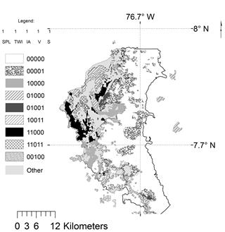
Source: The authors.
Figure 6 Location of levees, diversion points and combination of variables defining wetland potential. The color legend to the left includes those combinations where three variables or more are meeting the wetland condition, the color legend to the right two variables or less. SPL…Summary of piezometric levels, TWI…Topographic wetness index, IA… Observed inundated areas, V…Vegetation, S…Hydromorphic soils. To access the results of this study, see “Basemap” tab: http://geomatica.udem.edu.co/flexviewers/RioLeon/index.html
5. Conclusions
The binary decision method does not account for the fuzzy nature of wetlands, but does account for the relative importance of each variable to determine wetland potential. Hydrophytic vegetation and inundated areas are important to define marshes and swamps with a straightforward validation. Anytime a pixel in the data cube met one of these two conditions it was marked as a wetland pixel, disregarding the amount of variables meeting the wetland condition. Other areas could also be selected without these two variables because of the rule sum ≥ 2, which is the case for the coexistence of hydromorphic soils and TWI. This is an important rule to define wetland pixels when wetland ecosystems have been modified and no evidence of hydrophytic vegetation is available. This rule allows the inclusion of shrublands, cattle grazing ranches and highly modified banana and plantain crops within wetland boundaries. However, validation is difficult to obtain when natural vegetation is absent and no evidence of inundated areas is available. For instance, piezometric measurements provide strong evidence of the occurrence of inundated areas but statistical validation with independent sources is difficult to achieve. Hydromorphic soils was the variable less likely to correlate well with the current wetland status, especially to the east of the floodplain, where water level is controlled by agricultural practices and no other variables confirm the potential of wetland pixels. As a matter of fact, Cowardin et al. [1] did not consider drained hydromorphic soils as wetlands given the inability of these soils to support hydrophytes.
The lack of time series of flooding events and the low level of detail of soil maps are important sources of uncertainty when identifying potential areas for wetlands. It should be noted that the identification of inundated areas with closed forest canopies is difficult to achieve and optical remote sensing misses a fair amount of the ephemeral floods due to heavy cloud cover during the wet season. Additional sources of uncertainty are related to areas without monitoring wells [46] and the effect of drainage projects on surface runoff.
Soil fertility at the León River floodplains result in enormous pressure on natural vegetation and in conflicting objectives since land can only be assigned to use for agro industrial development or conservation. The impacts of banana crops are considered within the highest order of magnitude because of the extent, permanence and cost of the remedy. Further studies should consider the cost of the remedy for different land use categories and evaluate alternatives of productivity with sustainable development such as plantations of Prioira copaifera. As observed during field trips and through satellite images, fire is being used as a powerful tool to promote land use change from tropical forests to agriculture, aggravated by the fact that fire occurrence in coastal wetlands is considered a major source of greenhouse gas emissions [47].
Drastic modifications to surface hydrology were identified affecting the balance between erosion, transportation and deposition: levees, ditches and diversions of the watercourse. In addition to a complex network of ditches to drain crops, there are also two diversion sites transporting sediments to otherwise non-sediment prone ecosystems. Changing the distribution of sediments affects the mangroves as found by Restrepo and Alvarado [48], modifies the substrate of inundated forests [49], and accelerates sedimentation of floodplain lakes [50].
Since model variables are dynamic, it is recommended that the collection of inundated areas be improved, the density of piezometric levels increased, and a model of interaction between surface water and groundwater constructed. Modification of the surface hydrology through common practices such as the construction of levees, ditches and channels for water diversion is evident, but the cumulative effect on surface hydrology is difficult to assess.

